
Excel library
How to Make XLOOKUP Return All Matches? (5 Easy Methods)
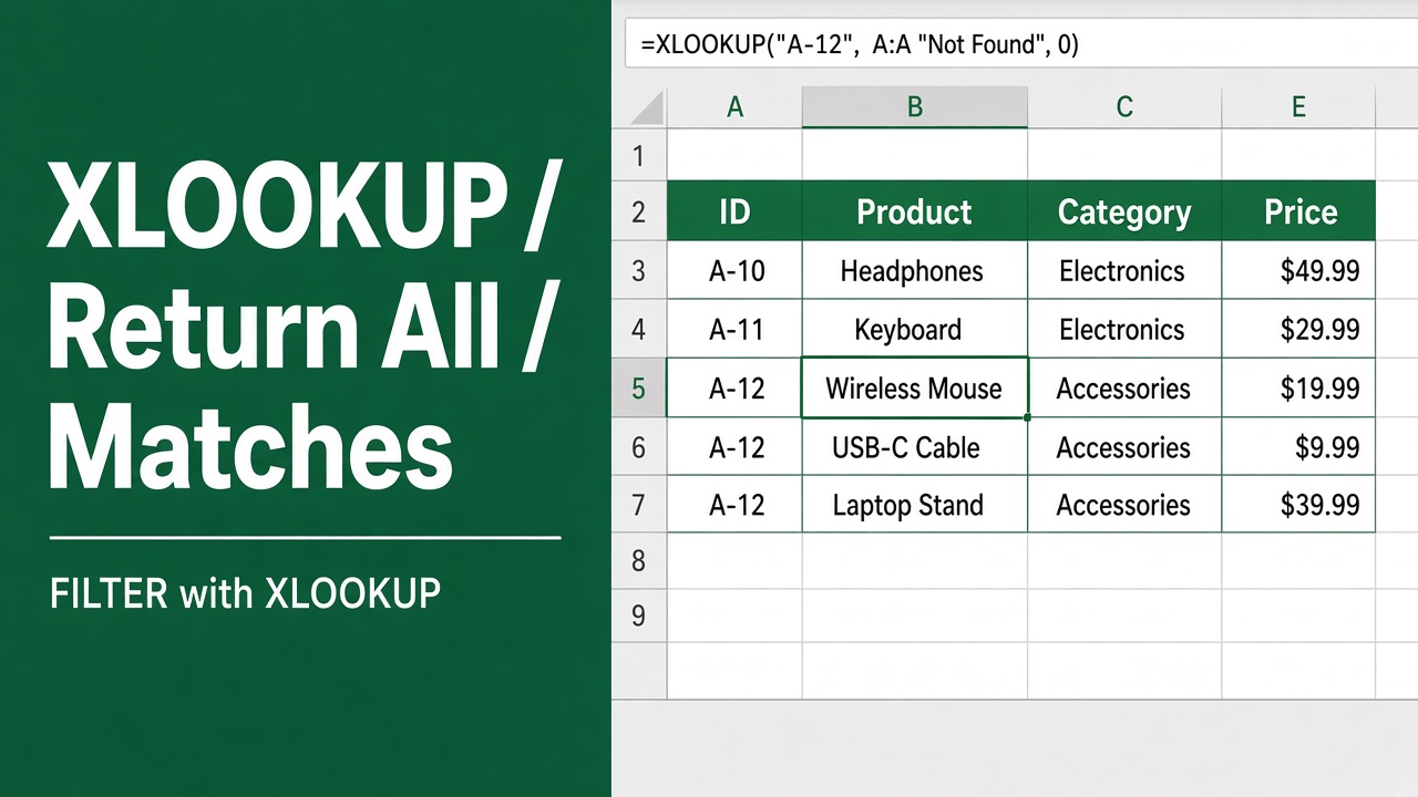
The XLOOKUP function in Excel is one of the most powerful tools for searching data. While it easily finds a single match, many users often ask: “How can I make XLOOKUP return all matches instead of just the first one?”
XLOOKUP only ever returns the first match. To get every match, use FILTER (Microsoft 365 and Excel 2021 or later):
=FILTER(B2:B100, A2:A100="Apple", "No match")The results spill down one per row. To put them all in one cell, separated by commas, use =TEXTJOIN(", ", TRUE, FILTER(B2:B100, A2:A100="Apple", "")). To return the address of a match rather than its value, see how to return a cell reference.
In this guide, we will walk you through practical methods to achieve this. You’ll learn formulas, supporting functions, and Excel tricks that allow you to extract multiple results from XLOOKUP in a clean and efficient way. If your lookup data is in another file, see how to use XLOOKUP with two workbooks.
Understanding XLOOKUP Basics
Before focusing on multiple matches, it’s important to understand what XLOOKUP does by default.
- Syntax of XLOOKUP:
=XLOOKUP(lookup_value, lookup_array, return_array, [if_not_found], [match_mode], [search_mode]) - Default behavior:
XLOOKUP finds the first matching value in the lookup array and returns the corresponding item from the return array. - Limitation:
It does not automatically return all matches when multiple entries exist.
For example:
If you search for “Apple” in a sales table, XLOOKUP will only bring back the first instance of Apple sales, not all rows.
Why You Need All Matches
In many real-world situations, returning only one value is not enough. Common cases include:
- Sales data: Finding all transactions for a specific customer.
- Inventory management: Listing all products from a category.
- Employee records: Returning all roles held by a person.
- Project tracking: Collecting all tasks assigned to a team member.
Getting all matches saves time, ensures accuracy, and eliminates the need for manual filtering.
Method 1: Using FILTER with XLOOKUP Logic
The FILTER function is the best way to simulate XLOOKUP returning multiple values.
Formula:
=FILTER(return_array, lookup_array=lookup_value, "Not Found")Example:
Imagine you have a table:
| Product | Sales |
|---|---|
| Apple | 120 |
| Banana | 90 |
| Apple | 150 |
| Orange | 200 |
| Apple | 180 |
To return all sales for Apple:
=FILTER(B2:B6, A2:A6="Apple", "Not Found")Result: {120;150;180}
Why this works:
FILTER checks all rows where the condition is true and returns every matching value. This makes it act like XLOOKUP for multiple matches.
Method 2: Get Only the First N Matches (or the Nth Match)
XLOOKUP can’t step through matches by itself; its last argument only sets the search direction or binary search. Instead, wrap FILTER with TAKE or INDEX.
First N matches:
=TAKE(FILTER(B2:B6, A2:A6="Apple"), 2)This returns the first 2 sales values for Apple: {120;150}. TAKE needs Microsoft 365 or Excel 2024.
Only the Nth match:
=INDEX(FILTER(B2:B6, A2:A6="Apple"), 3)This returns the 3rd Apple sale, 180. If there are fewer than 3 matches, INDEX returns #REF!, so wrap it in IFERROR if that can happen.
Method 3: Using TEXTJOIN
Method 3: Using TEXTJOIN with IF for a Single Cell Result
Sometimes, you may want all matches in one cell instead of separate rows. You can combine TEXTJOIN with an IF array.
Formula:
=TEXTJOIN(", ", TRUE, IF(A2:A6="Apple", B2:B6, ""))Result: 120, 150, 180
This creates a clean, comma-separated list of all values found.
Method 4: Dynamic Array Formula with INDEX & SMALL
For users who want a step-by-step extraction of multiple matches, INDEX with SMALL is a classic method.
Formula:
=INDEX(return_array, SMALL(IF(lookup_array=lookup_value, ROW(return_array)-MIN(ROW(return_array))+1), ROWS($A$1:A1)))- Works in older versions of Excel without FILTER.
- Requires pressing Ctrl+Shift+Enter if not using dynamic arrays.
- Each copy of the formula returns the next match.
Method 5: Using Power Query for Complex Data
If you work with large datasets, Power Query is more reliable.
Steps:
- Load your table into Power Query.
- Use a filter step to match the lookup value.
- Load the filtered results back into Excel.
This approach is perfect for advanced users managing thousands of rows.
Comparing Different Methods to Make XLOOKUP Return All Matches
Here’s a comparison table:
| Method | Ease of Use | Returns Multiple Matches | Works in Older Excel | Output Type |
|---|---|---|---|---|
| FILTER | Easy | Yes | No | Dynamic array |
| FILTER + TAKE / INDEX | Moderate | First N or Nth match | No | Dynamic array or single value |
| TEXTJOIN + IF | Moderate | Yes | Excel 2019 and later | Single cell text |
| INDEX + SMALL | Advanced | Yes | Yes | Multiple rows |
| Power Query | Advanced | Yes | Yes | Separate table |
Best Practices for Using XLOOKUP with Multiple Matches
- Use FILTER whenever possible – it’s the cleanest method for modern Excel.
- Combine with structured references if working in Excel tables.
- Be clear on output type – choose dynamic arrays vs. single-cell results depending on your needs.
- Check data consistency – spelling errors or hidden characters may cause missed matches.
- Test formulas with sample data before applying them to large reports.
Common Errors and Fixes
- #CALC! Error: FILTER returns #CALC! when nothing matches. Solution: fill in FILTER’s third argument, e.g.
"No match". - #VALUE! Error: Occurs in INDEX-SMALL arrays if ranges are inconsistent. Ensure arrays are the same size.
- Empty Results: Use TRIM or CLEAN functions to remove extra spaces in data.
Real-Life Example: Customer Orders Report
Imagine you run a retail business and want all orders for customer John.
| Customer | OrderID | Amount |
|---|---|---|
| John | 1001 | 250 |
| Mary | 1002 | 180 |
| John | 1003 | 320 |
| Paul | 1004 | 150 |
| John | 1005 | 400 |
Using FILTER:
=FILTER(B2:C6, A2:A6="John", "Not Found")Result:
| OrderID | Amount |
|---|---|
| 1001 | 250 |
| 1003 | 320 |
| 1005 | 400 |
This lets you quickly generate a customer order summary.
When to Avoid Forcing XLOOKUP to Return All Matches
- If you need aggregation (sum, average, count), use functions like SUMIFS, AVERAGEIFS, or COUNTIFS instead.
- If your dataset is very large, many FILTER formulas can slow down the workbook. Power Query or PivotTables are better.
- If working in older Excel (before Office 365), stick to INDEX-SMALL or helper columns.
Final Thoughts
While XLOOKUP does not directly return multiple results, using functions like FILTER, TEXTJOIN, or INDEX-SMALL unlocks that capability.
- Use FILTER for the most straightforward solution.
- Use TAKE or INDEX with FILTER when you only need the first few matches or one specific match.
- Use TEXTJOIN for a compact list in one cell.
- Use INDEX-SMALL or Power Query for compatibility with older Excel or large datasets.
With these methods, you can make XLOOKUP return all matches and manage your data more effectively.
Frequently Asked Questions
Can XLOOKUP return multiple matches in Excel?
By default, XLOOKUP only returns the first match. However, you can use supporting functions like FILTER or INDEX-SMALL to return all matches.
What is the best way to return all matches with XLOOKUP?
The easiest method is using the FILTER function. It allows you to extract every matching value dynamically without writing multiple formulas.
How do I get only the 2nd or 3rd match?
Wrap FILTER in INDEX, e.g. =INDEX(FILTER(B2:B6, A2:A6="Apple"), 2) for the 2nd match. XLOOKUP alone cannot return the nth match.
Can I list all XLOOKUP matches in a single cell?
Yes. By using TEXTJOIN with an IF formula, you can create a comma-separated list of all matching values in one cell.
Which method works in older versions of Excel?
If you are not using Office 365, you can use INDEX with SMALL to return multiple matches. This requires array formulas and works in older Excel versions.
When should I use Power Query instead of XLOOKUP?
Power Query is better for large datasets or when you need advanced filtering. It creates a separate table of all results instead of formulas inside cells.