
Excel library
How to Use the Index Match Excel Formula (The Right Way)
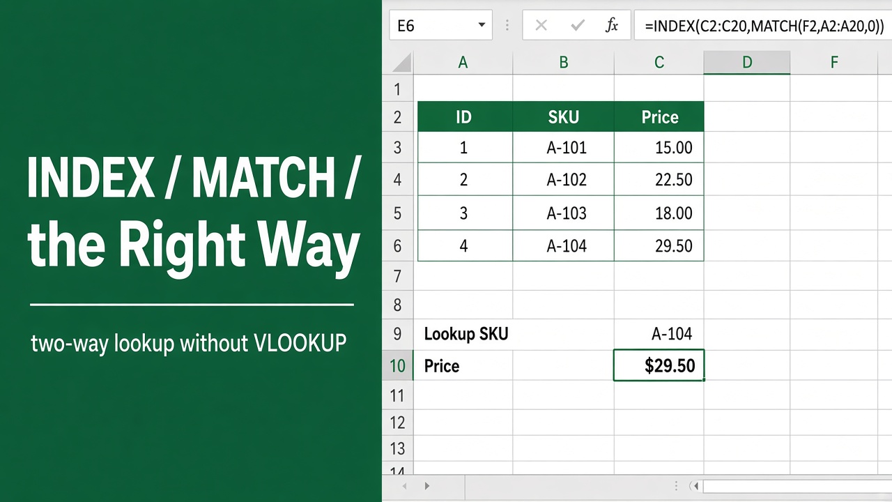
If you’re looking to master Excel formulas, the INDEX MATCH combination is a must-know. This powerful duo allows you to efficiently lookup and retrieve data from your spreadsheets, making it an essential tool for data analysis and reporting. In this comprehensive guide, we’ll learn everything about the INDEX MATCH formula, breaking down its components, explaining its usage, and providing practical examples to help you unlock its full potential.
Quick answer: use =INDEX(return_range, MATCH(lookup_value, lookup_range, 0)). MATCH finds the row of your value, and INDEX returns the value from that row in another column, including columns to the left.
What is the INDEX MATCH Formula?
The INDEX MATCH formula is a combination of two individual functions in Excel: INDEX and MATCH. Together, they create a dynamic and flexible way to search for and return specific values from a range of data based on given criteria.
The INDEX Function
The INDEX function returns a value from a specified cell or range of cells based on row and column numbers. Its syntax is as follows:
=INDEX(array, row_num, [column_num])- array: The range of cells containing the data you want to retrieve.
- row_num: The row number of the value you want to return.
- column_num (optional): The column number of the value you want to return. If omitted, the INDEX function assumes a one-dimensional array.
The INDEX function is particularly useful when you need to retrieve a value from a specific position within a range. For example, if you have a table of sales data and want to retrieve the sales figure for a particular month and product, you can use the INDEX function to specify the row and column numbers corresponding to the desired value.
The MATCH Function
The MATCH function searches for a specified value within a range of cells and returns its relative position. Its syntax is as follows:
=MATCH(lookup_value, lookup_array, [match_type])- lookup_value: The value you want to find in the lookup_array.
- lookup_array: The range of cells to search for the lookup_value.
- match_type (optional): Specifies the type of match to perform:
- 1 (default): Finds the largest value less than or equal to the lookup_value.
- 0: Finds an exact match for the lookup_value.
- -1: Finds the smallest value greater than or equal to the lookup_value.
The MATCH function is incredibly handy when you need to find the position of a specific value within a range. It eliminates the need for manual searching and allows you to dynamically locate data based on your criteria.
How to Use INDEX MATCH Formula
Now that we understand the individual components, let’s see how to combine them to create a powerful lookup formula.
Basic Syntax
The basic syntax for the INDEX MATCH formula is as follows:
=INDEX(return_range, MATCH(lookup_value, lookup_range, 0))- return_range: The range of cells containing the values you want to return.
- lookup_value: The value you want to find in the lookup_range.
- lookup_range: The range of cells to search for the lookup_value.
In this formula, the MATCH function is used to find the position of the lookup_value within the lookup_range. The result of the MATCH function is then used as the row_num argument for the INDEX function, which retrieves the corresponding value from the return_range.
Step-by-Step Example
Let’s consider a simple example to illustrate the usage of the INDEX MATCH formula. Suppose we have the following data table:
| Employee ID | Name | Department |
|---|---|---|
| 1001 | John Doe | Sales |
| 1002 | Jane Smith | Marketing |
| 1003 | Mike Johnson | Engineering |
To look up an employee’s department based on their ID, we can use the following formula:
=INDEX(C2:C4, MATCH(1001, A2:A4, 0))Here’s how it works:
- The MATCH function searches for the value “1001” in the range A2:A4 (Employee ID column) and returns its relative position (1, in this case).
- The INDEX function then uses the result from the MATCH function as the row_num argument and returns the value from the corresponding cell in the range C2:C4 (Department column).
The formula will return “Sales” as the result, which is the department for the employee with ID 1001.
Handling Errors and “Not Found” Values
When using the INDEX MATCH formula, there may be instances where the lookup_value is not found in the lookup_range. By default, this will result in an “#N/A” error. To handle such cases gracefully, you can wrap the formula with the IFERROR function.
The IFERROR function allows you to specify a custom value or message to return when an error occurs. Its syntax is as follows:
=IFERROR(value, value_if_error)- value: The formula or expression to evaluate.
- value_if_error: The value or message to return if an error occurs.
Here’s an example of using IFERROR with the INDEX MATCH formula:
=IFERROR(INDEX(Department, MATCH(1005, EmployeeID, 0)), "Employee not found")In this case, if the employee ID “1005” is not found in the EmployeeID column, the formula will return “Employee not found” instead of an “#N/A” error.
Advanced Techniques to Use INDEX MATCH Formula
Using Named Ranges
To make your INDEX MATCH formulas more readable and maintainable, you can use named ranges instead of cell references. Named ranges allow you to assign meaningful names to specific ranges of cells, making your formulas easier to understand and update.
For example, instead of using A2:A4 and C2:C4 in the previous example, you could define named ranges like “EmployeeID” and “Department”. The formula would then look like this:
=INDEX(Department, MATCH(1001, EmployeeID, 0))Using named ranges not only improves the readability of your formulas but also makes it easier to update the ranges if your data expands or moves to a different location in the spreadsheet.
Multiple Criteria Matching
In some cases, you may need to perform a lookup based on multiple criteria. You can do this by joining the criteria with & inside a single MATCH function. In Excel 2019 and older, confirm the formula with Ctrl + Shift + Enter; in Microsoft 365 a normal Enter works.
Let’s extend our previous example to include an additional criterion: the employee’s name. The data table now looks like this:
| Employee ID | Name | Department |
|---|---|---|
| 1001 | John Doe | Sales |
| 1002 | Jane Smith | Marketing |
| 1003 | Mike Johnson | Engineering |
| 1004 | John Doe | Marketing |
To look up an employee’s department based on both their ID and name, you can use the following formula:
=INDEX(Department, MATCH(1001&"John Doe", EmployeeID&Name, 0))Here, we concatenate the employee ID and name using the “&” operator to create a unique lookup value. The MATCH function then searches for this combined value in the concatenated range of EmployeeID and Name columns.
By using multiple criteria, you can ensure that the lookup is more specific and accurate, especially when dealing with duplicate values in one of the criteria ranges.
Performing Case-Sensitive Lookups
MATCH is not case-sensitive. It treats “JOHN DOE”, “john doe” and “John Doe” as the same value, so a normal INDEX MATCH already ignores capitalization and you don’t need LOWER or UPPER.
When capitalization matters, for example with product codes like “ab-100” and “AB-100”, use EXACT inside MATCH:
=INDEX(Department, MATCH(TRUE, EXACT("John Doe", Name), 0))EXACT compares the lookup value with every name and returns TRUE only for an exact, case-matching entry. MATCH then finds the position of that TRUE. In Excel 2019 and older, confirm this formula with Ctrl + Shift + Enter.
INDEX MATCH vs XLOOKUP: Which Should You Use?
If you have Excel for Microsoft 365, Excel 2021 or later, XLOOKUP does the same job in one function. The employee lookup from above becomes:
=XLOOKUP(1001, EmployeeID, Department, "Employee not found")| INDEX MATCH | XLOOKUP | |
|---|---|---|
| Works in | Every Excel version | Microsoft 365, Excel 2021 and later |
| Look up to the left | Yes | Yes |
| Exact match by default | No, add 0 as the match type | Yes |
| Built-in “not found” value | No, wrap in IFERROR | Yes, 4th argument |
| Multiple criteria | Array formula | Array formula, same idea |
Use INDEX MATCH when the file will be opened in Excel 2019 or older, or by people on different versions. Use XLOOKUP when everyone is on Microsoft 365; it is shorter and harder to get wrong.
Common Mistakes to Avoid While Working with INDEX MATCH
When working with INDEX MATCH formulas, be mindful of these common mistakes to ensure accurate results and avoid errors:
- Range Mismatch: Ensure that the lookup_range and return_range have the same number of rows. If they don’t match, you may encounter errors or incorrect results. Double-check your range references and make sure they cover the appropriate data ranges.
- Data Type Mismatch: Make sure the lookup_value and the values in the lookup_range have the same data type (e.g., text or numbers). If they don’t match, the MATCH function may return an incorrect position or an error. Ensure consistency in your data and use appropriate functions like TEXT or VALUE to convert data types if necessary.
- Forgetting the Match_Type: If you omit the match_type argument in the MATCH function, it defaults to 1, which performs an approximate match. Always specify 0 for an exact match unless you have a specific reason to use a different match type. Forgetting to set the match_type can lead to unexpected results or errors.
- Not Handling Errors: As mentioned earlier, it’s important to handle potential errors that may occur when the lookup_value is not found in the lookup_range. Use the IFERROR function or other error-handling techniques to provide meaningful feedback or default values in case of errors.
- Overcomplicating Formulas: While the INDEX MATCH formula is powerful, it’s important to keep your formulas as simple and readable as possible. Break down complex lookups into smaller, manageable steps and use named ranges or comments to document your formulas. This will make your spreadsheets easier to understand and maintain in the long run.
Final Thoughts
The INDEX MATCH formula is a powerful and versatile tool in Excel that enables you to perform complex lookups and data retrieval tasks. By mastering this formula, you can streamline your data analysis workflows, save time, and increase your productivity.
Remember to practice using INDEX MATCH in your own spreadsheets, experiment with different scenarios, and continuously refine your skills. As you become more comfortable with this formula, you’ll find yourself leveraging its power to solve increasingly complex data challenges.
FAQs
What is the difference between INDEX MATCH and VLOOKUP?
The main differences between INDEX MATCH and VLOOKUP are flexibility and performance. INDEX MATCH allows you to perform lookups in any direction and in non-contiguous ranges, while VLOOKUP always looks to the right of the lookup column. Additionally, INDEX MATCH is generally faster than VLOOKUP when working with large datasets.
Can INDEX MATCH handle multiple criteria lookups?
Yes, INDEX MATCH can handle multiple criteria lookups by joining the criteria with & inside one MATCH function, for example MATCH(1001&"John Doe", EmployeeID&Name, 0). This allows you to perform lookups based on multiple conditions, such as looking up an employee’s department based on both their ID and name.
How can I make my INDEX MATCH formulas more readable?
To make your INDEX MATCH formulas more readable, you can use named ranges instead of cell references. Named ranges allow you to assign meaningful names to specific ranges of cells, making your formulas easier to understand and update. This improves the readability and maintainability of your spreadsheets.
What should I do if the lookup value is not found in the lookup range?
If the lookup value is not found in the lookup range, the INDEX MATCH formula will return an “#N/A” error. To handle this gracefully, you can wrap the formula with the IFERROR function. The IFERROR function allows you to specify a custom value or message to return when an error occurs, such as “Value not found”.
Is INDEX MATCH case-sensitive?
No. MATCH ignores capitalization, so “john doe” matches “John Doe”. For a case-sensitive lookup, use =INDEX(Department, MATCH(TRUE, EXACT("John Doe", Name), 0)).