Easy Formula to Get Value from a Merged Cell in Excel

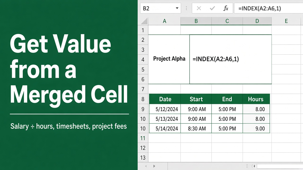
Have you ever been in a situation where you needed to extract data from a merged cell in Excel? Merged cells are a common feature in Excel spreadsheets, often used to create headings or improve the visual layout of data. However, working with merged cells can sometimes be challenging, especially when it comes to extracting values for calculations or analysis.

=LOOKUP(2, 1/($A$2:A2<>""), $A$2:A2)

In this article, we will explore the formula to get value from a merged cell in Excel in detail. We will discuss various methods and techniques to tackle this issue effectively.

Understanding Merged Cells in Excel

Before we learn about extracting values from merged cells, let’s take a moment to understand what merged cells are in Excel. When you merge two or more adjacent cells in Excel, you are essentially combining them into a single cell that spans the same area as the merged cells. This can be useful for creating headers, labels, or improving the visual presentation of your data.

While merged cells can be visually appealing and help organize data, they can also create challenges when it comes to using functions or formulas that require individual cell references. Excel treats a merged cell as a single entity, making it tricky to work with them in certain scenarios.

Where Excel Stores a Merged Cell’s Value

When cells are merged, Excel keeps the value only in the top-left cell of the merged area. The other cells are empty. So if A2:A5 are merged and show “North”, then =A2 returns North, but =A3, =A4 and =A5 return 0 (an empty cell).

That is why lookups, filters, sorting and SUMIFS go wrong with merged cells: every row except the first looks blank. The fix is to give each row its value.

Formula: Return the Merged Value on Every Row

With vertically merged labels in column A starting at A2, enter this in a helper column on row 2 and copy it down:

=LOOKUP(2, 1/($A$2:A2<>""), $A$2:A2)

• $A$2:A2 grows by one row as the formula is copied down.
• 1/($A$2:A2<>"") gives 1 for filled cells and an error for blanks.
• LOOKUP(2, …) can’t find 2, so it returns the last non-blank value above, which is the value of the merged block the row belongs to.

Each row now shows North, North, North… and you can use the helper column in VLOOKUP, SUMIFS or a pivot table. The formula works in every version of Excel and doesn’t need Ctrl + Shift + Enter.

Unmerge and Fill the Blanks (No Formula)

To fix the data permanently:

1. Select the merged column and click Home > Merge & Center to unmerge it. Only the top cell of each block keeps the value.
2. With the column still selected, press F5, click Special, choose Blanks, and click OK.
3. Type =, press the Up Arrow (so the formula points to the cell above), then press Ctrl + Enter. Every blank fills with the value above it.
4. Copy the column and use Paste Special > Values to replace the formulas with text.

Using Power Query: Fill Down

If the data is loaded with Power Query (Data > From Table/Range), merged cells arrive as a value followed by nulls. Select the column, go to Transform > Fill > Down, and click Close & Load. The fill is repeated automatically on every refresh.

Using a VBA Function

For a function you can point at any cell inside a merged block, add this to a module (Alt + F11 > Insert > Module) and use =MergedValue(A4):

Function MergedValue(cell As Range) As Variant
    MergedValue = cell.MergeArea.Cells(1, 1).Value
End Function

MergeArea is the whole merged block the cell belongs to, and .Cells(1, 1) is its top-left cell, where the value is stored. Save the file as .xlsm.

Tip: to center a title across columns without merging, select the cells, press Ctrl + 1, and choose Center Across Selection on the Alignment tab. It looks the same but keeps every cell usable.

Final Thoughts

Working with merged cells in Excel can present challenges, particularly when you need to extract values for calculations, analysis, or reporting purposes. However, by employing techniques such as the CONCATENATE function, INDEX function with CHOOSE, VBA macros, and Power Query, you can overcome these challenges and effectively extract values from merged cells in Excel.

The ability to extract data from merged cells opens up new possibilities for data manipulation and analysis in Excel. Whether you choose to use formulas, VBA macros, or data transformation tools like Power Query, exploring these methods will equip you with the skills to navigate and work with merged cells efficiently.