
Excel library
How to Use Excel Formulas to Get Values Based on Cell Color?
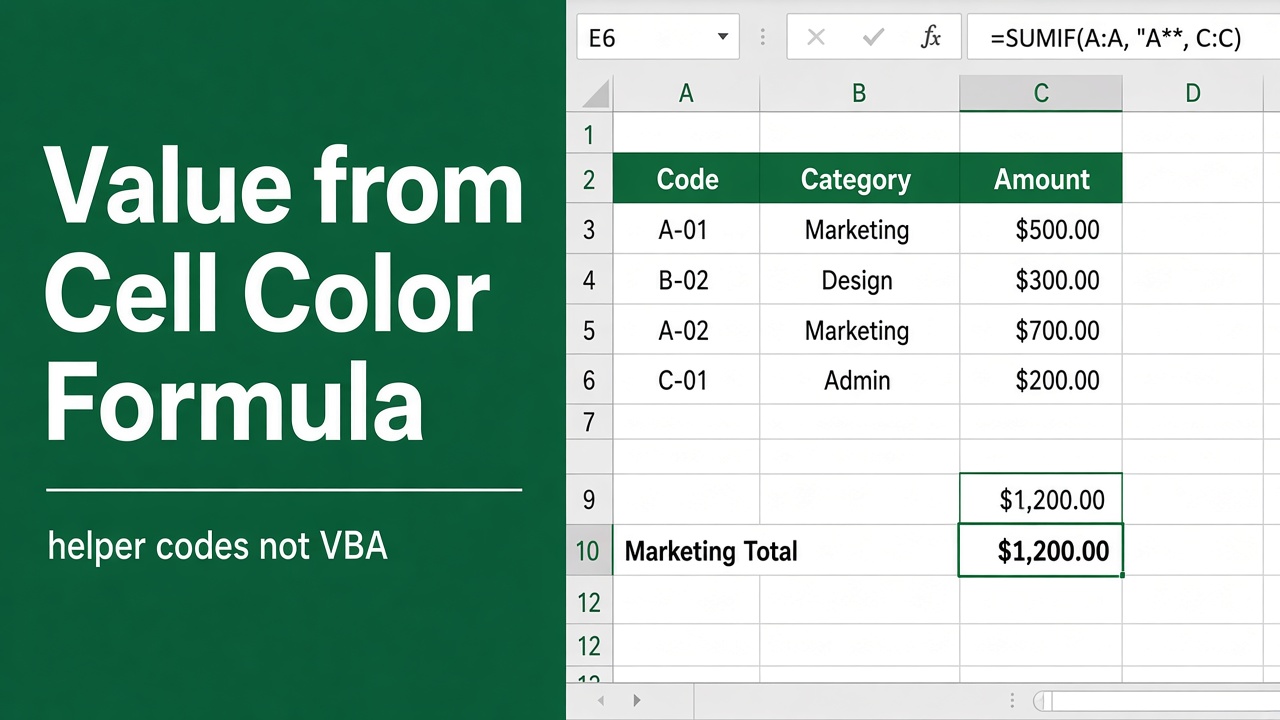
Have you ever wanted to extract values from colored cells in Microsoft Excel? Maybe you have a spreadsheet where certain cells are highlighted in red, green, yellow, or another color to indicate something about their values. Fortunately, it’s possible to write Excel formulas that return values based on cell colors.
Excel has no formula that reads cell color directly. The quickest reliable way:
- Turn on Data > Filter and choose Filter by Color on the colored column.
- Use
=SUBTOTAL(109, B2:B100)to sum only the visible (colored) rows,101to average, or103to count.
For a total that doesn’t need filtering, use the SumByColor VBA function in Method 3. If the colors come from conditional formatting, skip color entirely and sum with the rule’s own condition in SUMIFS.
In this article, we’ll cover step-by-step how to set up formulas in Excel that allow you to pull out values from colored cells. You’ll learn multiple methods to achieve this, including using Excel’s conditional formatting feature along with formulas like SUMIF, COUNTIF, AVERAGEIF and more. By the end, you’ll have several options for retrieving values based on the interior shading color of cells in any Excel worksheet.
Why Get Values from Colored Cells in Excel?
There are many scenarios where you may want to extract cell values by color in Excel:
- Analyzing data where colors represent categories, priorities, or statuses
- Creating reports that show totals/averages of colored subsets of data
- Identifying key datapoints that have been manually highlighted
- Checking which colored cells contain certain numeric thresholds
- Summarizing results from worksheets that use color-coding
Whatever your reasons for needing to get values from colored cells, Excel’s built-in tools and formulas provide multiple ways to accomplish this. The best method will depend on your specific spreadsheet setup and goals.
Method 1: Filter by Color and Use SUBTOTAL
One straightforward way to sum values in colored cells is to:
- Select your data range
- Go to Data > Filter to enable filters
- Click the filter arrow and select Filter by Color
- Choose the color of the cells you want to sum
- With the colored rows filtered, enter a SUBTOTAL formula like:
=SUBTOTAL(9,B2:B100)The “9” in this formula includes only visible cells in the sum. The filtered color will be the only visible rows included.
To get the average of colored cells instead of the sum, use “101” instead of “9” in the SUBTOTAL formula. For a count of colored cells, use “2” or “102”.
This method works well for quickly summing, averaging or counting the values in a specific cell color that you select using the Filter feature. However, if you want more dynamic formulas that automatically adjust based on color without manual filtering, try the next techniques.
Pros and Cons of Filtering and SUBTOTAL
Filtering by color and using SUBTOTAL is a good choice when you need a one-time calculation of values from a specific colored subset of your data. It allows you to visually select the exact color you want and instantly see the matching cells.
However, the downside is that it’s a manual process that must be redone any time your data or colors change. The SUBTOTAL result does update when you change values, but you have to re-apply the filter to count a different color or pick up recolored cells.
Method 2: Use GET.CELL in a Helper Column
GET.CELL is an old Excel 4 macro function that can return a cell’s fill color number. It only works inside a defined name, so you use it through a helper column:
- Click C2 (the helper column, in the same row as your first value in B2).
- Go to Formulas > Define Name. Name it FillColor and in Refers to enter
=GET.CELL(38,B2)without $ signs, so the name always reads the cell to its left. - In C2 enter
=FillColorand copy it down. Each row shows a color number, for example 3 for red or 6 for yellow. - Sum by color with
=SUMIF(C2:C100, 6, B2:B100). Use AVERAGEIF or COUNTIF the same way.
Pros and Cons of GET.CELL Formulas
It needs no VBA code, but the file must be saved as .xlsm because GET.CELL is a macro function. Changing a cell’s color doesn’t trigger a recalculation, so press F9 after recoloring. It also reads only colors you applied by hand; colors from conditional formatting return the cell’s original fill.
Method 3: Custom VBA Functions
For the most dynamic option that will automatically sum/average/count cell values based on colors without any conditional formatting or named formulas, you can use custom VBA functions. If you cannot use macros, see how to build a formula based on cell color without VBA.
Here are the steps:
- Go to the Visual Basic Editor (Alt+F11)
- Right-click your workbook name, select Insert > Module
- Paste this code into the Module:
Function SumByColor(rng As Range, colorNum As Long) As Double
  Dim total As Double
  Dim cell As Range
  Application.Volatile
  For Each cell In rng
    If cell.Interior.Color = colorNum Then
        total = total + cell.Value
    End If
  Next cell
  SumByColor = total
End Function- Save and return to your Excel worksheet
- Enter a formula like:
=SumByColor(B2:B100, RGB(255, 0, 0))
That formula will sum all values in red cells. The RGB function specifies the color to match. You can look up RGB color codes to find the one you need.
To get the average of colored cells with VBA instead of the sum, modify the custom function like this:
Function AverageByColor(rng As Range, colorNum As Long) As Double
  Dim total As Double
  Dim count As Long
  Dim cell As Range
  Application.Volatile
  For Each cell In rng
    If cell.Interior.Color = colorNum Then
        total = total + cell.Value
        count = count + 1
    End If
  Next cell
  If count > 0 Then AverageByColor = total / count
End Function
For a count of colored cells, use:
Function CountByColor(rng As Range, colorNum As Long) As Double
  Dim count As Long
  Dim cell As Range
  Application.Volatile
  For Each cell In rng
    If cell.Interior.Color = colorNum Then
        count = count + 1
    End If
  Next cell
  CountByColor = count
End Function
Then enter formulas like:
=AverageByColor(C2:C100, RGB(0, 255, 0))
=CountByColor(A2:A200, RGB(255, 255, 0))
Pros and Cons of VBA Functions
Using custom VBA functions to retrieve values by cell color is incredibly flexible and efficient. You don’t need to set up any conditional formatting, named ranges, or helper columns. Your formulas are compact and readable.
Plus, VBA gives you the full power of looping through each individual cell to check its color and value. So it works with any fill color you apply by hand. It can’t see colors that come from conditional formatting, because those don’t change the cell’s own fill. Recoloring a cell doesn’t trigger a recalculation, so press F9 after changing colors.
The only disadvantage is that you must enable macros in your workbook for the custom functions to run. And if you want to modify them or create your own, you’ll need some understanding of Excel VBA programming. But once set up, the formulas are simple to use.
Summary
To recap, here are the main ways to get values based on cell color in Excel:
| Method | Pros | Cons |
|---|---|---|
| Filter & SUBTOTAL | Easy to set up, flexible color selection | Manual process, doesn’t auto-update |
| GET.CELL helper column | No VBA code, works with SUMIF/COUNTIF | Needs .xlsm, press F9 after recoloring |
| VBA Functions | Simplest formulas, fully automatic | Requires enabling macros, VBA knowledge |
The best approach will depend on your spreadsheet and how often you need to pull data from colored cells. But with these techniques, you can unlock lots of possibilities for dynamically extracting values based on color formatting in Excel.
Whether you need to analyze data, create reports, check thresholds, or summarize results, these formulas will let you quickly retrieve values from cells of a specific color. Experiment with each method to find the one that works best for your needs!
FAQs
What is the easiest way to sum values in colored cells in Excel?
The easiest way to sum values in colored cells is to use Excel’s Filter feature to filter by color, then use a SUBTOTAL formula to sum the visible cells. This method allows you to quickly select the color you want and get a sum of the matching cells.
How can I create a formula that automatically updates when cell colors change?
No formula updates the moment a color changes, because recoloring doesn’t make Excel recalculate. The closest option is a GET.CELL helper column or a VBA function with Application.Volatile, followed by F9 after you change colors.
What is the most flexible way to retrieve values from colored cells in Excel?
The most flexible way to retrieve values from colored cells is to use custom VBA functions. With VBA, you can write functions that loop through ranges and check the interior color of each cell individually. This works with any fill color applied by hand, but not with colors from conditional formatting.
Can I use these methods to get the average or count of colored cells, not just the sum?
Yes, all of these methods can be adapted to find the average or count of colored cells as well. For filtering, use “101” in SUBTOTAL for average or “2” for count. With GET.CELL, use AVERAGEIF or COUNTIF instead of SUMIF. And for VBA, modify the function to calculate an average or count instead of a sum.
What are the pros and cons of using VBA functions to sum cells by color?
The main advantages of VBA functions are flexibility and efficiency. Your formulas will be simple and will work with any coloring method. However, the cons are that you must enable macros and you may need some VBA knowledge to set up or modify the functions.