How to Insert a Row in Excel Without Breaking Formulas?

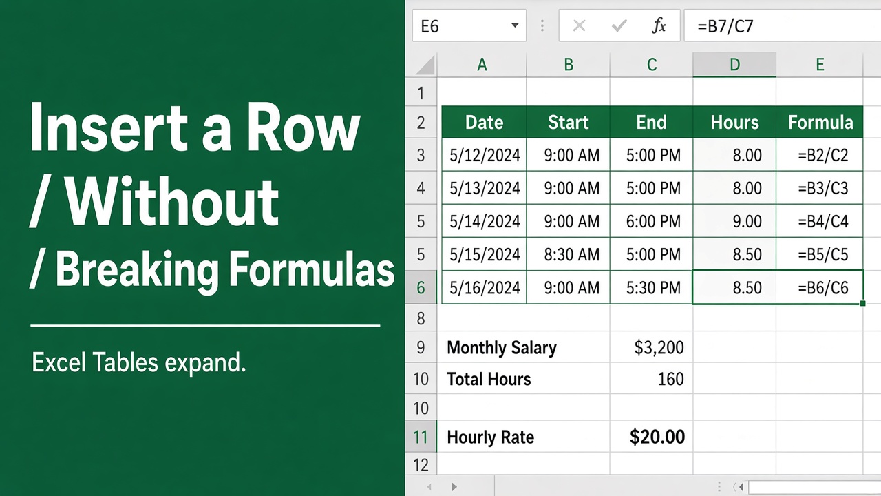
Are you trying to insert a new row in Microsoft Excel but finding that it’s breaking your carefully crafted formulas? This common issue can be frustrating, especially if you have a complex spreadsheet with many interlinked calculations. Luckily, there are several easy methods to add rows in Excel while preserving your formulas intact. In this article, we’ll show you exactly how to insert a row in excel without breaking formulas step-by-step.

Key Takeaways

• Excel does update references when you insert a row inside a range: =SUM(B2:B10) becomes =SUM(B2:B11) automatically.
• Formulas break when you insert a row just below the end of a range (the new row is left out) or when the new row needs formulas of its own.
• Converting your data to an Excel Table solves both problems: ranges grow and formulas fill into new rows automatically.
• For a total row under a plain range, =SUM(B2:INDEX(B:B,ROW()-1)) always includes every row above it.
• Dynamic named ranges also grow with the data, but Tables are simpler.

Why Inserting Rows Can Break Formulas in Excel

Inserting a row in the middle of a range is safe. If B11 holds =SUM(B2:B10) and you insert a row at row 5, Excel changes the formula to =SUM(B2:B11) and moves it to B12. Relative and absolute references ($B$2) both shift this way.

Problems come from these situations instead:

• Inserting at the edge of a range. If you insert a row directly above the total row (below B10), the new row is outside B2:B10, so the total ignores it. Excel sometimes extends the range for you, but not reliably.
• The new row has no formulas. An inserted row is empty, so columns that normally hold formulas (such as Amount = Qty × Price) stay blank until you fill them in.
• Running totals and “row above” formulas. A formula like =C4+B5 in the row below the new one keeps pointing at the old row, skipping the new one.
• References typed as text. Ranges inside INDIRECT("B2:B10") or hard-coded in VBA never adjust.

Method 1: Insert Rows Inside the Range, Then Fill the Formulas

For a plain range, insert new rows somewhere between the first and last data row rather than below the last one:

1. Right-click the row number where the new row should go (not the total row) and choose Insert.
2. Select the cell above the new row in each formula column together with the new cell, and press Ctrl + D to fill the formula down.
3. Check the total: click it and confirm its range now includes the new row.

This works, but it is easy to forget step 2 in a large sheet.

Method 2: Make the Total Row Always Include Every Row Above It

If you keep a total directly under a list and often add rows just above it, replace the fixed range with one that ends at the row above the total:

=SUM(B2:INDEX(B:B,ROW()-1))

ROW()-1 is the row just above the formula, and INDEX turns it into a cell reference. However many rows you insert above the total, the sum always runs from B2 to the last row before it.

Method 3: Use Excel Tables for Automatic Formula Updates

An even more powerful solution is to convert your data range into an Excel Table:

1. Select any cell in your data range.
2. Go to the Insert tab on the ribbon and click the Table button.
3. Confirm the range selection and check the “My table has headers” box if your data has header rows. Click OK.
4. Excel will format your data as a Table with banded rows, filter buttons, and automatic updates to formulas.
5. Any formulas referencing the Table will now use special Table syntax like =SUM(Table1[Column1]).
6. When you insert a row anywhere in the Table, the formulas will instantly include the new row in their calculations without breaking.

Using Tables is an excellent best practice in Excel. It not only prevents broken formulas when inserting rows but also provides other benefits like easy sorting, filtering, and cleaner formula syntax.

Here’s an example Table formula:

=SUM(Table1[[#Data],[Column1]])

This formula sums all values in Column1 of Table1, excluding the header row. The [[#Data]] specifier represents the data rows.

Method 4: Use Dynamic Named Ranges

For advanced Excel users, you can also leverage dynamic named ranges to create robust formulas:

1. Select your data range and define a named range (e.g. “MyData”) using the Name Box to the left of the formula bar.
2. Rather than referencing the range directly in formulas, reference the named range instead. For example: =SUM(MyData).
3. Open the Name Manager (Formulas tab > Name Manager) and edit the named range.
4. Change the Refers To field to use the OFFSET function to make the range dynamic, such as:

=OFFSET(Sheet1!$B$2,0,0,COUNTA(Sheet1!$B:$B)-1,1)

This formula defines MyData as starting in B2 and extending down to the last contiguous value in column B.

5. Now use the named range MyData in your formulas, and they will automatically expand to include any inserted rows within the data.

With a dynamic named range, your formula like =SUM(MyData) will always sum the entire contiguous data in column B, even as you add or remove rows.

Tips for Avoiding Broken Formulas When Inserting Rows

Beyond the specific methods outlined above, here are some general tips to minimize formula breakage:

• Plan ahead: Think about potential insertions/deletions when first building your sheet and formulas.
• Use cell references strategically: Relative, mixed, and absolute references behave differently when inserting rows.
• Embrace Tables: Convert data to Tables by default to allow easy expansion and formula updates.
• Avoid hard-coded ranges: Don’t manually define SUM(B2:B10). Let Excel define the range dynamically with a Table or OFFSET.
• Use Named Ranges: Named ranges are easier to work with than cell references and can be made dynamic.
• Check for errors: After inserting rows, do a quick scan of your formulas to look for any #REF! or #VALUE! errors.

By following these tips and best practices, you can build robust Excel spreadsheets that handle new rows gracefully.

Final Thoughts

Inserting a new row in Excel doesn’t have to spell disaster for your formulas. By using absolute references, Tables, named ranges, or other dynamic techniques, you can ensure your calculations update correctly when the spreadsheet structure changes.

The key is to plan ahead, reference cells strategically, and leverage Excel’s built-in tools for flexibility. With a bit of forethought and the right approach, you can build powerful spreadsheets that adapt seamlessly as you add or remove data.

FAQs