How to Sort Months in Excel Pivot Table: Easy Guide

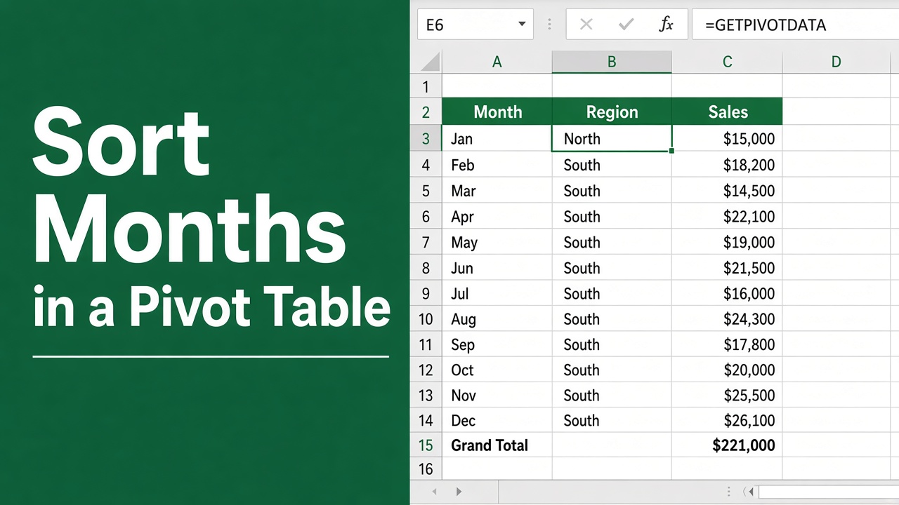
If you’ve ever tried to sort months chronologically in an Excel Pivot Table, you may have run into issues with the months being sorted alphabetically instead (April, August, December, etc.). Luckily, there is an easy fix to sort the months in proper calendar order in your Pivot Table. This article will walk you through the steps to chronologically sort months in an Excel Pivot Table so you can easily analyze your data by month.

Why Months Get Sorted Alphabetically in Pivot Tables

When you add a field containing month names to a Pivot Table in Excel, the months will automatically get sorted in alphabetical order by default. This is because Excel treats the month names as text strings and applies an A-to-Z sort, rather than recognizing them as dates and sorting them chronologically.

While an alphabetical sort may work fine in some cases, it makes the data much harder to analyze when you want to view metrics and trends over time with the months in proper calendar order from January to December.

For example, if you have a Pivot Table summarizing monthly sales data, an alphabetical sort will place April’s numbers at the top, followed by August, December, February, and so on. This makes it very difficult to compare the sales performance from one month to the next in a meaningful way. By sorting the months chronologically instead, you can easily scan down the list from January to December to spot upward or downward trends over the course of the year.

Steps to Sort Months in Chronological Order

Excel has built-in custom lists for month names (January–December and Jan–Dec), and pivot tables use them when sorting. So the fix is usually to switch that option back on and sort again:

1. Right-click the pivot table and choose PivotTable Options.
2. On the Totals & Filters tab, tick Use Custom Lists when sorting and click OK.
3. Right-click any month name and choose Sort > Sort A to Z. The months now run January to December.

If a month is still out of place, it was probably dragged there by hand. Click the Row Labels arrow, choose More Sort Options, pick Ascending (A to Z) by the month field, then click More Options, untick Sort automatically every time the report is updated if needed, and choose the January, February, March… list under First key sort order.

Additional Tip: the month names must match the list exactly. “Sept” or “january ” with a trailing space won’t be recognized, so clean them with TRIM or Find & Replace first.

Best Option: Use Real Dates and Group by Month

If your data has actual dates rather than month names, you don’t need a month column at all:

1. Put the Date field in Rows. In Microsoft 365, Excel often groups it by Years and Months automatically.
2. If it doesn’t, right-click a date, choose Group, select Months (and Years if the data covers more than one year), and click OK.

Grouped months always sort in calendar order, and new data joins the right month when you refresh.

Sorting Months in Pivot Tables Using a Formula

Another approach is a helper column with the month number, which forces the order even if custom lists are off:

1. In your source data, insert a new column next to the month names, for example with the header MonthNo.
2. Enter =MONTH(1&A2), where A2 holds the month name, and copy it down. “1March” is read as a date, so this returns 3.
3. Refresh the pivot table and drag MonthNo into Rows above the month name field.
4. Switch to Design > Report Layout > Show in Tabular Form and turn off subtotals for MonthNo. The months now follow the number order; you can hide the MonthNo column if you like.

Pivot Tables Built on the Data Model or Power Pivot

If the pivot table was created with Add this data to the Data Model ticked, or from Power Pivot, custom lists are ignored and the steps above will not fix the order. Tell the model which column to sort the month names by instead:

1. Open Power Pivot > Manage (enable the Power Pivot add-in under File > Options > Add-ins > COM Add-ins if the tab is missing).
2. In the table with the month names, add a calculated column for the month number, for example =MONTH('Sales'[Date]). If you only have month names, use =MONTH(DATEVALUE("1 " & 'Sales'[Month])).
3. Select the month name column, then choose Home > Sort by Column.
4. Sort the month name column by the new month number column and click OK.
5. Back in Excel, refresh the pivot table (Data > Refresh All). The months now appear January to December wherever that field is used.

Sort Months in Fiscal Year Order

To start the year in a month other than January, for example April to March, add your own custom list and sort by it:

1. Go to File > Options > Advanced and click Edit Custom Lists (under General).
2. In List entries, type the months in the order you want, one per line (April, May, June … March), and click Add, then OK.
3. In the pivot table, click the Row Labels arrow > More Sort Options > Ascending (A to Z) by the month field.
4. Click More Options, untick Sort automatically every time the report is updated, choose your new list under First key sort order, and click OK twice.

Custom lists are saved on your computer, not in the workbook, so someone else opening the file will see the order you set but will need the list themselves to re-sort it.

Troubleshooting Month Sorting Issues

If you tried the steps above and your months are still not sorting chronologically, here are a few things to double-check:

• Make sure the source data has the month names spelled correctly and consistently (e.g. not a mix of “January” and “Jan”)
• If using the formula method, verify that the formula is filled down correctly for all rows and returns a valid month number for each cell
• Check for any extra spaces, punctuation or other characters in the month name cells that could interfere with sorting
• Ensure you have followed all the steps in the correct order and clicked “OK” to apply the changes

If you’ve checked all these things and still can’t get your months to sort chronologically, try creating a new Pivot Table from scratch with just the essential columns and double-check the sorting steps as you go. If the issue persists, there may be a problem with your source data that needs to be investigated further.

Final Thoughts

By following the steps outlined above, you can easily sort the months in proper chronological order in an Excel Pivot Table. Whether you use the built-in month sorting option or create your own custom sort order with a formula, this will allow you to analyze and visualize your data by month more effectively.

Remember, the key steps are:

1. Turn on Use Custom Lists when sorting (PivotTable Options > Totals & Filters) and sort the months A to Z
2. Better still, keep real dates in the source and group the date field by Months
3. For a Data Model or Power Pivot table, use Sort by Column with a month number column
4. For a fiscal year, add your own month list and choose it under More Sort Options

With your months sorted from January to December, you’ll be able to scan through the data and identify patterns, trends and insights more easily. Whether you’re analyzing sales figures, website traffic, budget data or other metrics, putting the months in calendar order is an important step in creating an effective Pivot Table.

FAQs