
Excel library
How to Hide Zero Values in Excel Chart? (9 Easy Methods)
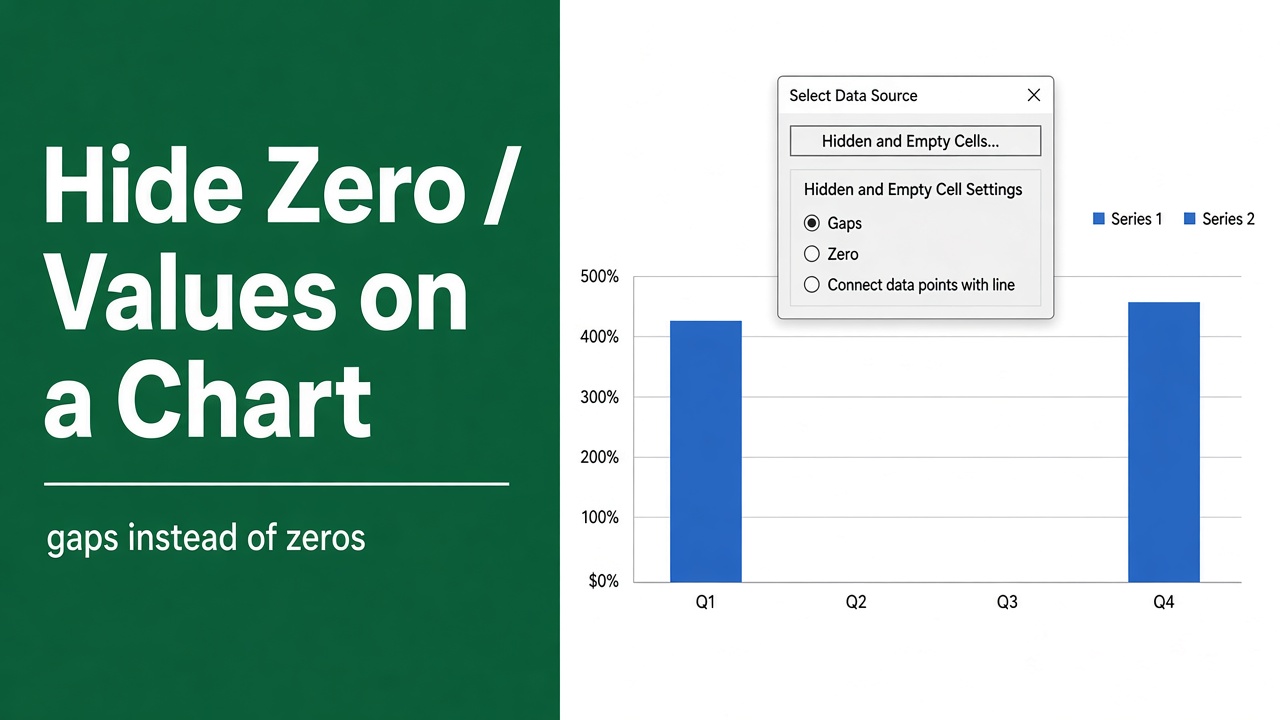
Microsoft Excel is one of the most powerful spreadsheet tools for data visualization. But when you are working with charts, zero values can sometimes make your chart look misleading or cluttered. For example, a line chart might drop to the baseline for zero values, or a column chart may show unnecessary empty bars. This can distract your audience from the actual data trends.
- Column or bar chart: zero bars are already invisible; to hide the “0” labels, format the data labels with the custom number format
0;-0;;@. - Line chart: change the source to
=IF(B2=0, NA(), B2). Excel doesn’t plot #N/A, so the line no longer drops to zero. - Remove the category completely: filter the zero rows out of the data; charts skip hidden rows by default.
Fortunately, Excel provides multiple ways to hide zero values in charts without losing your underlying data. In this guide, we’ll explore different methods step by step.
Why You Might Want to Hide Zero Values
Before moving to the techniques, let’s quickly understand why hiding zero values can improve chart readability:
- Cleaner visualizations – Zero values may distort the chart by pulling lines down to the baseline or adding extra bars.
- Focus on real data – Hiding zeroes ensures that trends and patterns are clearer.
- Improved reporting – When sharing reports, charts without zeros look more professional and easier to interpret.
- Accurate storytelling – Eliminating irrelevant data points helps the audience focus on key insights.
Method 1: Use Filter to Exclude Zero Values
The easiest way to prevent zeros from appearing in your chart is by filtering them out from the dataset.
Steps:
- Select your data range.
- Go to the Data tab and click Filter.
- Use the dropdown filter on the column that contains values.
- Uncheck 0 from the list.
- The chart updates straight away, because charts skip hidden rows by default. (If it doesn’t, check that Show data in hidden rows and columns is off under Select Data > Hidden and Empty Cells.)
Key Points:
- This method removes zeros from the dataset entirely.
- It is useful when zero values are not relevant for your analysis.
Method 2: Use IF Formula to Replace Zeros with Blank
Another effective approach is using an IF function to replace zero values with blank cells.
Example Formula:
=IF(A2=0,"",A2)This formula checks if a cell contains a zero. If yes, it replaces it with a blank cell; otherwise, it keeps the original value.
How It Works:
- In a column or bar chart, the “” result is plotted as zero, which draws no bar, so the zero simply disappears. Data labels may still show 0; hide them with Method 4.
- In a line chart, “” is text, and Excel plots text as zero, so the line still drops to the baseline. Use
NA()(Method 5) for line charts instead.
Example:
| Original Data | Formula Result |
|---|---|
| 25 | 25 |
| 0 | (blank) |
| 40 | 40 |
This makes the chart look cleaner and prevents lines or columns from falling to zero.
Method 3: Change Zero Display Settings
Excel also allows you to hide zeros directly in the worksheet without altering the formulas.
Steps:
- Go to the File menu and click Options.
- Select Advanced.
- Scroll to the section Display options for this worksheet.
- Uncheck the option Show a zero in cells that have zero value.
Notes:
- This only hides zeros in the cells. The chart still plots them as zero, so combine it with another method.
- It does not delete or replace the actual value, only hides the display.
Method 4: Format Data Labels to Hide Zeros
If you only want to remove zero values from data labels (but keep the chart structure intact), formatting is the best choice.
Steps:
- Click your chart.
- Select the Data Labels you want to edit.
- Right-click → Format Data Labels.
- Choose Number → Custom.
- Use a custom format like:
0;-0;;@This format hides zero values from appearing in labels.
Benefit:
- Keeps the chart points intact but prevents unnecessary zero labels.
Method 5: Use NA() Function to Skip Zeros
If you’re creating a line chart or scatter chart, replacing zeros with #N/A values ensures Excel completely skips plotting them.
Formula Example:
=IF(A2=0,NA(),A2)Why It Works:
- Excel doesn’t plot #N/A values at all, so no point or marker appears for them.
- By default, a line chart connects the points on either side of an #N/A, so the line skips over the missing value instead of dropping to zero.
- If you want a visible gap instead, open Select Data > Hidden and Empty Cells, tick Show #N/A as an empty cell (Microsoft 365), and choose Gaps.
Example:
| Original | Formula Output |
|---|---|
| 20 | 20 |
| 0 | #N/A |
| 35 | 35 |
In the chart, the line will not dip to zero; it joins the points on either side instead, unless you set #N/A to show as a gap (see Method 6).
Method 6: Adjust Chart Options for Empty Cells
The Hidden and Empty Cells settings control how a chart handles truly empty cells. They don’t change how zeros are plotted: a 0 is always drawn as 0.
Steps:
- Right-click the chart and choose Select Data.
- Click Hidden and Empty Cells.
- Choose how to show empty cells: Gaps (a break in the line), Zero (drop to the baseline) or Connect data points with line.
- In Microsoft 365, tick Show #N/A as an empty cell so #N/A values from Method 5 follow the same choice.
Best Use:
- Combine it with Method 5: turn zeros into #N/A with a formula, then decide here whether they show as gaps or connected lines.
Method 7: Use Conditional Formatting in the Data Table
If your chart pulls from a table, you can use conditional formatting to hide zeros before they reach the chart.
Steps:
- Select the dataset.
- Go to Home > Conditional Formatting > New Rule.
- Choose Format only cells that contain.
- Set the condition: Cell Value = 0.
- Change font color to white (or background color).
Limitation:
- This only hides zeros visually in the table, not in the chart itself.
- Combine with other methods for best results.
Method 8: Chart a Filtered Copy of the Data (Microsoft 365)
In Microsoft 365, FILTER can build a copy of the data without the zero rows, and the chart can use that copy. With categories in A2:A20 and values in B2:B20:
=FILTER(A2:B20, B2:B20<>0)- Enter it in an empty area, such as D2, and build the chart from the spilled result.
- To make the chart grow and shrink with the result, define names that refer to the spill, e.g.
=Sheet1!$D$2#, and use them in the chart’s series. - Zero rows are left out entirely, so they take no space on the category axis.
Method 9: VBA Macro to Hide Zero Data Labels
To hide zero labels on every series of a chart in one go, select the chart and run this macro. It applies the same number format as Method 4:
Example Code:
Sub HideZeroLabels()
    Dim s As Series
    For Each s In ActiveChart.SeriesCollection
        If s.HasDataLabels Then s.DataLabels.NumberFormat = "0;-0;;@"
    Next s
End Sub
Advantage:
- Fixes all series at once instead of formatting each label set by hand.
- The data itself is untouched, so the macro can’t damage your numbers.
Comparing the Methods to Hide Zero Values in Excel Chart
Here’s a comparison of methods you can use depending on your needs:
| Method | Best For | Effect on Data |
|---|---|---|
| Filter zeros | Simple charts | Removes zeros |
| IF formula with blanks | Column and bar charts | Zero bars disappear; lines still drop to 0 |
| Worksheet settings | General worksheets | Only hides display |
| Format data labels | Labels only | Does not affect values |
| NA() function | Line/Scatter charts | Point skipped, line connects over it |
| Hidden & empty cell settings | Empty cells and #N/A | Gaps, zero or connected line |
| Conditional formatting | Worksheet display | Visual only |
| FILTER copy (Microsoft 365) | Removing zero categories | Zero rows left out |
| VBA macro for labels | Many series or charts | Labels only |
Tips for Cleaner Excel Charts
- Use consistent formatting – Avoid mixing methods within the same chart.
- Test on different chart types – Some methods work better on line charts, while others suit column charts.
- Consider audience needs – Sometimes showing zeros is necessary for accuracy, especially in financial reporting.
- Keep backup data – If using formulas to replace zeros, store the original dataset separately.
Final Thoughts
Knowing how to hide zero values in Excel charts can make your reports cleaner, more professional, and easier to interpret. Depending on your scenario, you can use quick fixes like filters and display settings, or advanced approaches like NA() functions, dynamic ranges, or VBA macros.
The key is choosing the right method for your chart type and reporting needs. Once you apply these techniques, your charts will highlight the data that truly matters and present a clearer story to your audience.
Frequently Asked Questions
How do I remove zero values from an Excel chart?
You can remove zero values by using the IF formula to replace zeros with blanks, applying filters to exclude zero values, or using Excel’s NA() function so zeros are skipped in charts.
Can I hide zeros without changing the original data?
Yes. You can adjust Excel worksheet display settings to hide zeros or format data labels so zeros do not appear, while keeping the actual data intact.
Which method works best for line charts with zero values?
For line charts, the NA() function is best because it replaces zero with #N/A. Excel doesn’t plot those points, so the line no longer drops to zero; it connects across them, or leaves a gap if you choose that under Hidden and Empty Cells.
Can I hide zeros only in data labels but still show chart points?
Yes. You can format data labels with a custom number format such as 0;-0;;@ to hide zero labels while keeping the chart points visible.
Is there a way to automate hiding zeros in Excel charts?
Yes. A short VBA macro can apply the 0;-0;;@ label format to every series in a chart. For the plotted values themselves, use =IF(B2=0, NA(), B2) in the source data.
Will filtering out zeros affect my calculations?
If you use filters to exclude zeros, they won’t be included in the chart or calculations based on the filtered data. To keep calculations intact, use formulas or formatting instead.