How to Enable Distinct Count in Excel Pivot Table?

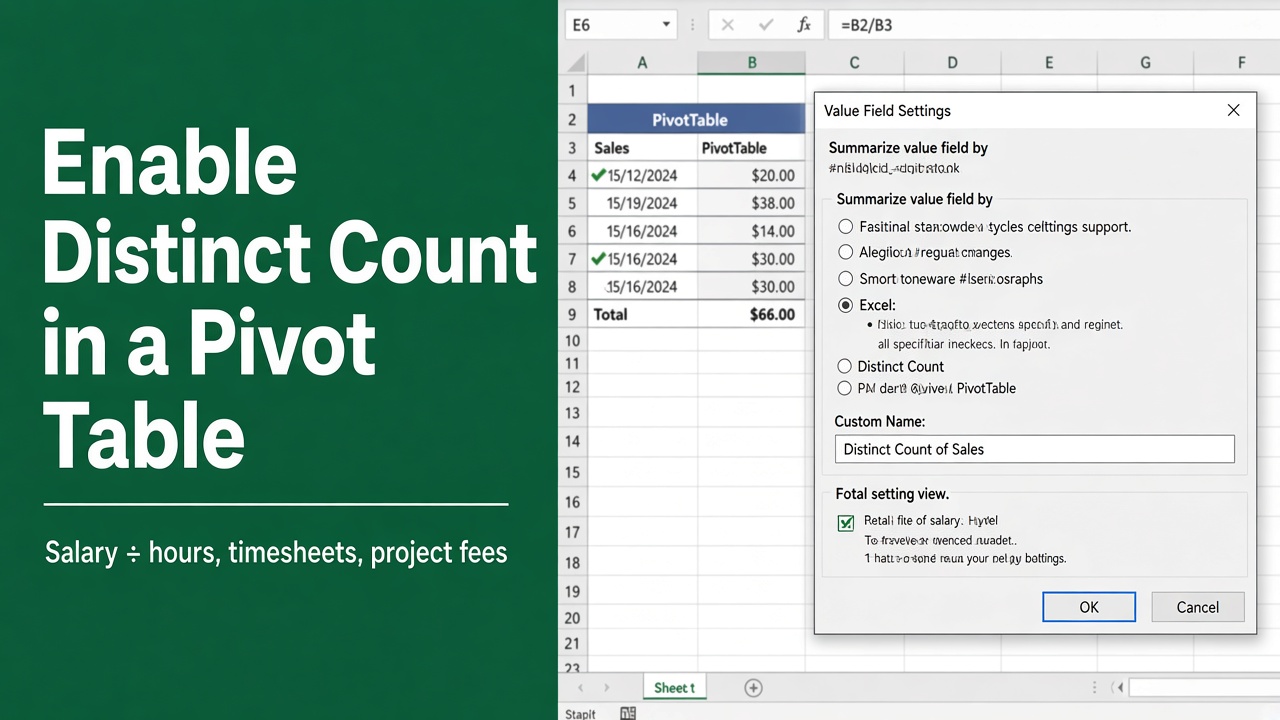
Pivot Tables in Excel are a powerful tool for summarizing and analyzing large datasets. A common task that Excel users might encounter is calculating the distinct count or unique count of values in a dataset. By default, Excel does not display the distinct count option in Pivot Tables, but there is a straightforward way to enable it.

In this article, we will guide you through the steps to activate and utilize the distinct count feature in Excel Pivot Tables, enhancing your data analysis capabilities.

Introduction to Distinct Count in Pivot Tables

Before diving into the steps, let’s understand what distinct count is and why it’s essential. Distinct count, often referred to as unique count, is a function that counts how many unique values are present in a dataset.

This is particularly useful when you need to count items without duplication. For example, if you want to know how many unique clients are purchasing from your store, rather than how many total transactions occurred.

Excel Versions and Distinct Count Availability

Distinct count in Pivot Tables is available in Excel 2013 and later versions. For users with Excel 2010 or earlier, distinct count might not be directly available, and different approaches, such as using additional formulas or tools, might be necessary. This guide focuses primarily on Excel 2013 and newer versions.

Excel for Mac does not support the Data Model, so Distinct Count doesn’t appear in Mac pivot tables. On a Mac with Microsoft 365, use =COUNTA(UNIQUE(A2:A100)) instead. If the range can contain blank cells, use =COUNTA(UNIQUE(FILTER(A2:A100, A2:A100<>""))) so the blank isn’t counted as a value.

Enabling Distinct Count in Excel Pivot Tables

To enable distinct count in Excel’s Pivot Tables, follow these detailed steps:

Step 1: Prepare Your Data

Ensure that your data is well-organized, ideally in a table format (using the Excel Table feature under the “Insert” tab). Proper data organization ensures accuracy when executing distinct counts.

Data Formatting Tips:

• Ensure no empty rows or columns within your data range.
• Eliminate or correct errors in data, such as misspellings or inconsistent entries, which can affect distinct counts.

Step 2: Insert a Pivot Table

1. Select any cell within your dataset.
2. Go to the Insert tab on the Ribbon.
3. Click on PivotTable.
4. In the Create PivotTable dialog box, choose whether you want the Pivot Table report to be placed in a new worksheet or an existing worksheet.
5. Click OK to create the Pivot Table.

Step 3: Enable the “Add this data to the Data Model” option

In Excel 2013 and later, when creating a Pivot Table, you have the option to add your data to the Data Model, which is crucial for enabling distinct counts.

1. Follow the steps to insert a Pivot Table.
2. In the Create PivotTable dialog box, check the box that says “Add this data to the Data Model” before clicking OK.
3. Adding data to the Data Model allows you to utilize more advanced data analysis features in Excel, including distinct count.

Step 4: Using Distinct Count in the Pivot Table

1. Once your Pivot Table is created, drag the field for which you want the distinct count into the Values area.
2. Click on the field’s dropdown in the Values area, and select “Value Field Settings.”
3. In the Value Field Settings dialog, under “Summarize value field by,” scroll down and select “Distinct Count.”
4. Click OK to apply the settings.

Practical Tips and Use Cases for Distinct Count in Excel Pivot Tables

Utilizing the distinct count feature in Excel Pivot Tables can significantly enhance your data analysis capabilities. Let’s explore some practical tips and scenarios where distinct count can be particularly useful.

Practical Tips for Using Distinct Count

Tip 1: Double-Check Your Data Model

When working with distinct counts, it’s crucial to ensure that your data model accurately reflects the relationships and hierarchies in your data. Misrepresented data can lead to inaccurate counts and misleading results.

Tip 2: Combine with Other Pivot Table Features

Distinct count becomes even more powerful when used in combination with other Pivot Table tools and features such as filters, slicers, and calculated fields. This integration allows for dynamic and flexible data analysis.

Tip 3: Refresh Your Pivot Table

Remember to refresh your Pivot Table whenever you make changes to the underlying data. This ensures that your Pivot Table reflects the most current data, including the distinct counts.

Use Cases for Distinct Count

Use Case 1: Analyzing Customer Behavior

Scenario: You have a database with multiple transactions per customer. Using distinct count in a Pivot Table, you can easily determine the number of unique customers who made purchases during a specific period. This insight can help in customer retention strategies and marketing campaigns.

Steps:

1. Add Month (or Region) to the Rows area.
2. Add Customer ID to the Values area and set it to Distinct Count. Each row now shows how many different customers bought in that month.
3. Optionally, add Date to the Filters area to analyze specific periods.

Use Case 2: Inventory Management

Scenario: In inventory management, it’s crucial to understand how many unique products are in stock, sold, or ordered. Distinct count can provide this information quickly and accurately.

Steps:

1. Add Status (such as “In Stock” or “Sold”) to the Rows area.
2. Add Product Code to the Values area and set it to Distinct Count. You get the number of different products in each status, not the number of stock lines.
3. Add Warehouse or Category to Columns to break it down further.

Use Case 3: Identifying Unique Entries in Data Cleansing

Scenario: During data cleansing, identifying unique entries can help in recognizing errors or duplicates. Distinct count in a Pivot Table can facilitate this process, making it efficient to pinpoint issues. To merge those duplicates into one row, see how to combine duplicates in a pivot table.

Steps:

1. Add the field (e.g., email addresses, employee IDs) to the Values area twice: set one to Count and the other to Distinct Count.
2. If Count is higher than Distinct Count, the column has duplicates. The difference is the number of extra entries.
3. To see which values repeat, add the same field to the Rows area, keep only the Count value, and sort it largest to smallest. Any row with a count above 1 is a duplicate.

These use cases illustrate how distinct count can be a versatile tool in various data analysis scenarios, providing deeper insights and aiding in decision-making processes.

Advanced Techniques and Troubleshooting for Distinct Counts in Excel Pivot Tables

While distinct count is a potent feature in Excel Pivot Tables, users might sometimes face challenges or require more sophisticated analysis methods. This section will cover advanced techniques and provide troubleshooting tips to enhance your experience with distinct counts.

Advanced Techniques for Distinct Count

Technique 1: Combining Distinct Count with Calculated Fields

Pivot tables that use the Data Model don’t allow calculated fields; the option is greyed out. Use a measure instead. For instance, you might want to calculate the average number of transactions per unique customer.

Steps:

1. In the PivotTable Fields pane, right-click your table name and choose Add Measure.
2. Name it (for example “Transactions per Customer”) and enter a formula such as =COUNTROWS(Sales)/DISTINCTCOUNT(Sales[Customer ID]), where Sales is your table name.
3. Click OK and tick the new measure to add it to Values.

Technique 2: Using Distinct Count with Power Pivot

For users with access to Excel’s Power Pivot add-in, distinct count can be implemented more robustly. Power Pivot allows for more complex data models and can handle larger datasets efficiently.

Steps:

1. Load your data into Power Pivot.
2. Create a Pivot Table from the Power Pivot window.
3. Use the distinct count in the same way as in a regular Pivot Table, benefiting from the enhanced processing power and advanced data modeling features of Power Pivot.

Troubleshooting Common Issues

Issue 1: Distinct Count Option Not Available

Solution: Ensure that you have added your data to the Data Model while creating the Pivot Table. Without integrating into the Data Model, the distinct count option will not be visible.

Issue 2: Inaccurate Distinct Count Results

Solution: Check for any discrepancies in your data entries. Typos, extra spaces, or inconsistent use of upper and lower case can lead to incorrect distinct counts. Tools like Trim or Proper in Excel can help clean up your data.

Issue 3: Performance Issues with Large Datasets

Solution: Distinct counts can be resource-intensive, especially with large datasets. Consider using Excel’s Power Pivot feature for handling large volumes of data more efficiently, or try to simplify your data model by removing unnecessary calculations and data fields.

Best Practices for Maintaining Efficient Pivot Tables with Distinct Count

• Regularly update and refresh your Pivot Table to reflect the latest data and calculations.
• Use slicers and filters to manage the visibility of specific data points, reducing the load on Excel’s processing.
• Keep your data clean and well-organized, and ensure that the data model accurately represents the relationships within your data.

By mastering these advanced techniques and troubleshooting common problems, you can leverage the full power of distinct counts in Excel Pivot Tables. This capability will not only enhance your data analysis tasks but also provide deeper insights and more actionable data for business decisions.