
Excel library
How to Display Text in Excel Pivot Table – Tips & Tricks
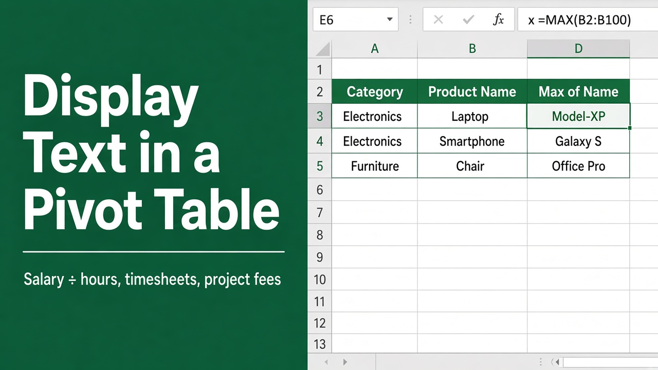
Displaying text in an Excel pivot table is a common requirement for many users. Pivot tables are a powerful tool for analyzing and summarizing large amounts of data, but they can be tricky to work with when it comes to displaying text values. In this article, we will explore various methods to display text in an Excel pivot table, making it easier for you to present your data effectively.
The Values area only counts or sums, so text there turns into numbers. To show text, drag the text field into Rows and set Design > Report Layout > Show in Tabular Form and Repeat All Item Labels. To join several text values into one cell (like “Apple, Banana”), add the data to the Data Model and use a CONCATENATEX measure (Method 3).
Understanding Pivot Tables and Text Values
Before we dive into the methods of displaying text in a pivot table, let’s briefly discuss what pivot tables are and how they handle text values.
What is a Pivot Table?
A pivot table is a tool in Excel that allows you to summarize and analyze data from a larger table or range. It enables you to quickly aggregate, sort, and filter data based on various criteria, making it easier to identify patterns and trends.
Pivot tables are particularly useful when dealing with large datasets, as they can help you:
- Summarize data by different categories or groups
- Calculate totals, averages, and other statistical measures
- Identify relationships and trends within your data
- Create interactive reports that can be easily updated with new data
How Pivot Tables Handle Text Values
By default, pivot tables are designed to work with numeric data. When you add a text field to a pivot table, Excel will attempt to summarize the data by counting the number of occurrences of each unique text value. This can lead to unexpected results, especially if you want to display the actual text values instead of a count.
For example, consider the following dataset:
| Product | Category |
|---|---|
| Apple | Fruit |
| Banana | Fruit |
| Carrot | Vegetable |
| Spinach | Vegetable |
If you create a pivot table with “Category” in the rows area and “Product” in the values area, Excel will display the count of products for each category, like this:
| Category | Count of Product |
|---|---|
| Fruit | 2 |
| Vegetable | 2 |
However, if you want to display the actual product names instead of the count, you’ll need to use one of the methods discussed in the following sections.
Method 1: Put the Text Field in Rows, Not Values
The Values area can only calculate numbers, so text placed there becomes a count. Pivot tables show text perfectly well in the Rows area, and with the right layout they look like a normal table:
- Drag Category and then Product into Rows.
- Go to Design > Report Layout > Show in Tabular Form, then Design > Report Layout > Repeat All Item Labels.
- Set Design > Subtotals > Do Not Show Subtotals.
Each product now appears as text next to its category, and you can still add numeric fields such as Sales to Values alongside it.
| Category | Product |
|---|---|
| Fruit | Apple |
| Fruit | Banana |
| Vegetable | Carrot |
| Vegetable | Spinach |
Why not “Max”? A common tip is to summarize the text field by Max, but pivot tables ignore text when calculating, so Max of a text field returns 0, not a word.
Method 2: Show Number Codes as Words with a Number Format
If each cell should show one of a few fixed labels, such as a status, store a number in a helper column in the source data (1 = Low, 2 = Medium, 3 = High) and let the number format display the word:
- Add the helper column (for example with
=MATCH(C2, {"Low","Medium","High"}, 0)) and put it in the pivot table’s Values area, summarized by Max. - Right-click a value, choose Number Format > Custom, and enter:
[=1]"Low";[=2]"Medium";"High"
The cells hold 1, 2 or 3 but display Low, Medium or High. A custom format can hold two conditions plus a default, so this works for up to three labels.
Method 3: Using a CONCATENATEX Measure (Data Model)
To list every matching text value in one cell, such as “Apple, Banana”, use a measure. This works in Excel for Windows with any Microsoft 365 or Excel 2016+ edition that has the Data Model; you don’t need to open the Power Pivot window.
- Select your data and go to Insert > PivotTable. Tick Add this data to the Data Model and click OK.
- In the PivotTable Fields pane, right-click the table name and choose Add Measure.
- Name it and enter a DAX formula such as the one below, where Table1 is your table name.
- Put Category in Rows and tick the new measure to add it to Values.
=CONCATENATEX(VALUES(Table1[Product]), Table1[Product], ", ")VALUES lists each product once, so repeated names appear only once per category. Your pivot table would now display:
| Category | Product Names |
|---|---|
| Fruit | Apple, Banana |
| Vegetable | Carrot, Spinach |
Method 4: A Formula Alternative in Microsoft 365 (GROUPBY)
If you only need the summary and not an actual pivot table, Microsoft 365’s GROUPBY function can join the text for you. With products in A2:A5 and categories in B2:B5:
=GROUPBY(B2:B5, A2:A5, ARRAYTOTEXT, , 0)It returns each category with its products joined by commas, and updates as the data changes. The 0 leaves out the grand-total row.
Best Practices for Displaying Text in Pivot Tables
When working with text in pivot tables, keep these best practices in mind:
- Use clear and concise labels: Ensure that your text values are easily understandable and consistent throughout your data.
- Avoid long text values: Long text values can make your pivot table difficult to read and navigate. Consider abbreviating or summarizing text where possible.
- Use filters: Leverage pivot table filters to focus on specific subsets of your data, making it easier to analyze text values.
- Format your pivot table: Apply appropriate formatting, such as bolding, italicizing, or coloring, to highlight important text values and make your pivot table more visually appealing.
- Choose the right method: Consider the size of your dataset, the complexity of your analysis, and your own skill level when deciding which method to use for displaying text in your pivot table.
Troubleshooting Common Issues
If you encounter issues while trying to display text in a pivot table, consider these troubleshooting tips:
- Check your source data: Ensure that your source data is properly formatted and free of errors or inconsistencies.
- Refresh your pivot table: If you make changes to your source data or pivot table settings, be sure to refresh the pivot table to see the updated results.
- Verify your calculations: Double-check any formulas or calculations you are using to ensure they are correctly referencing the desired text fields.
- Consult Excel documentation: If you are unsure about a specific function or feature, refer to the official Microsoft Excel documentation or seek guidance from online forums and communities.
- Test with a smaller dataset: If you’re working with a large or complex dataset, try testing your methods on a smaller subset of the data to isolate any issues.
Real-World Examples
To better understand how displaying text in pivot tables can be useful, let’s look at a few real-world examples:
- Sales Analysis: A retail company wants to analyze its sales data by product category and region. By displaying the product names in a pivot table, they can quickly identify the top-selling products in each category and region, helping them make informed decisions about inventory management and marketing strategies.
- Customer Feedback: A software company collects customer feedback through surveys. By creating a pivot table that displays the comments alongside the corresponding ratings, they can easily identify common themes and issues, allowing them to prioritize improvements and address customer concerns.
- Inventory Tracking: A manufacturing company needs to keep track of its inventory levels across multiple warehouses. By using a pivot table to display the product names and quantities for each warehouse, they can quickly identify which products need to be restocked and optimize their inventory distribution.
Final Thoughts
Displaying text in an Excel pivot table can be achieved through various methods, each with its own advantages and limitations. By understanding how pivot tables handle text values and applying the appropriate method for your specific needs, you can effectively present your data and gain valuable insights.
Remember to keep your pivot tables clean, concise, and well-formatted to ensure maximum readability and usability. With practice and experimentation, you’ll become proficient in displaying text in pivot tables and leveraging the full potential of this powerful Excel feature.
Frequently Asked Questions (FAQ)
1. Which method should I use to display text in my pivot table?
The choice of method depends on your specific needs, the size of your dataset, and your level of expertise with Excel. If you just need the text next to each category, put it in the Rows area with tabular layout (Method 1). For a few fixed labels, use number codes with a custom format (Method 2). To list several text values in one cell, use a CONCATENATEX measure (Method 3).
2. Can I combine multiple methods to display text in a pivot table?
Yes, you can combine different methods to achieve your desired result. For example, you might show some text fields in the Rows area and use a CONCATENATEX measure for another field that has several values per row.
3. What if I want to display text in a pivot chart?
Displaying text in a pivot chart follows similar principles to displaying text in a pivot table. You can use the methods discussed in this article to ensure that your pivot table displays the correct text values, and then create a pivot chart based on that pivot table.
4. How can I format the text displayed in my pivot table?
To format the text in your pivot table, select the cells containing the text and use the formatting options in the “Home” tab of the Excel ribbon. You can change the font, size, color, and other attributes to make your text more visually appealing and easier to read. In addition to formatting individual cells, you can also adjust the overall layout of the pivot table, including wrapping text in pivot table cells to ensure that all content is fully visible. By customizing the appearance of your pivot table, you can create a more professional and user-friendly presentation of your data. Experiment with different formatting options to find the best design for your specific needs. Wrapping text in pivot table cells can also help to improve the overall organization and clarity of the data.
5. Can I display text in a pivot table created from an external data source?
Yes, you can display text in a pivot table created from an external data source, such as a database or another spreadsheet. However, you may need to refresh your pivot table after making changes to the external data source to ensure that the text values are up-to-date.