
Excel library
How to Check Excel Pivot Table Source: A Complete Guide
Have you ever looked at a pivot table in Microsoft Excel and wondered where the underlying data came from? Pivot tables are powerful tools for summarizing and analyzing large datasets, but it’s important to be able to trace the source data to ensure accuracy and make updates as needed. In this article, we’ll walk through step-by-step how to check the source data for an Excel pivot table.
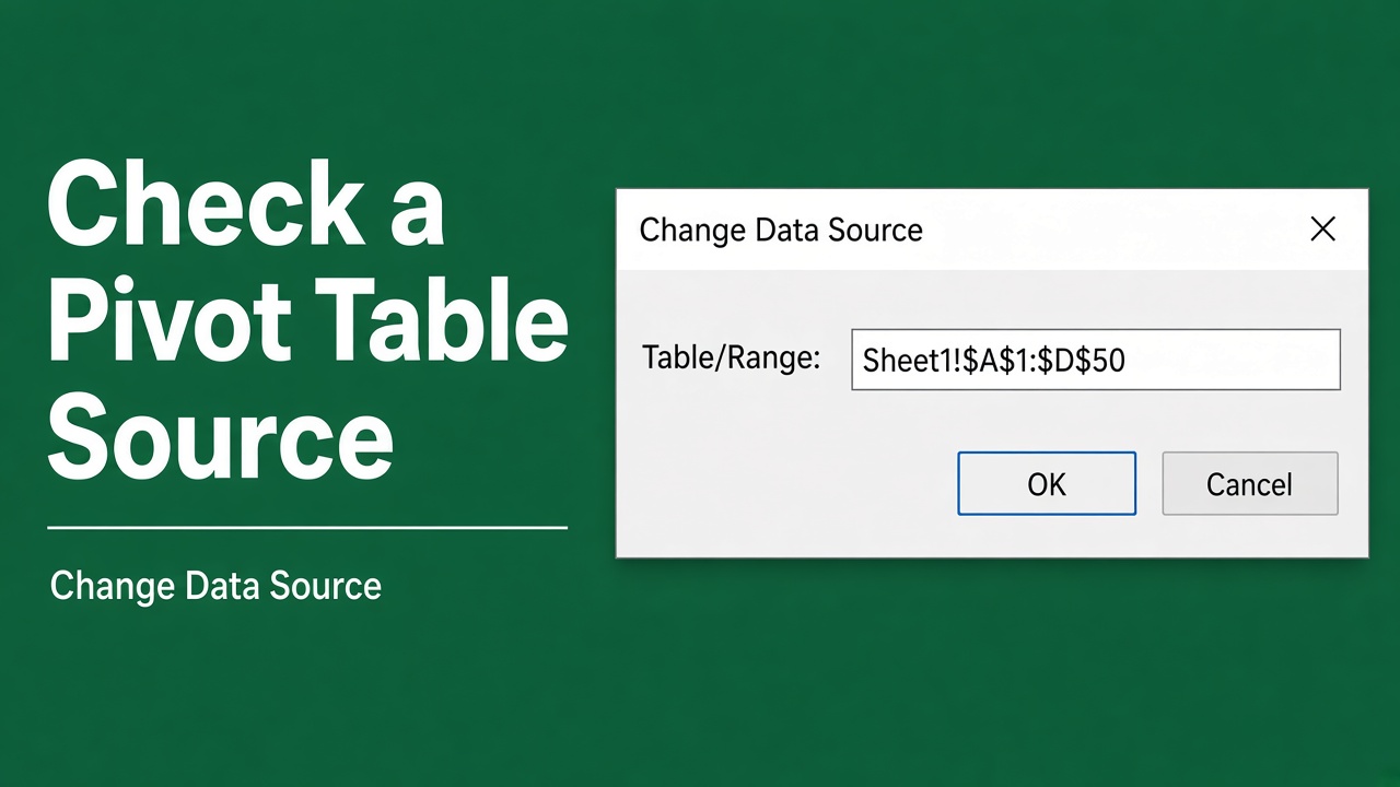
Click any cell in the pivot table, go to PivotTable Analyze > Change Data Source, and read the Table/Range box. It shows the table name or range (e.g. Data!$A$1:$D$200) the pivot table uses, and Excel outlines that range on the sheet. Click Cancel to close without changing anything.
Why Check the Pivot Table Source?
Before learning about the process, let’s discuss a few key reasons why you might need to check the source data behind a pivot table:
- To verify the accuracy of the summarized data
- To update the source data and refresh the pivot table
- To troubleshoot issues or unexpected results in the pivot table
- To copy or move the source data to another location
Checking the Pivot Table Source
Now let’s discuss how to actually go about checking where your pivot table data is pulled from. We’ll break it down into a series of steps.
Step 1: Select Any Cell in the Pivot Table
The first step is to click on any cell inside the pivot table that you want to trace the source for. This can be a value cell or a row/column heading cell. Just be sure you’ve selected a cell that is part of the actual pivot table.
Step 2: Go to the PivotTable Analyze Tab
With a pivot table cell selected, a PivotTable Analyze tab appears on the ribbon (called Analyze in Excel 2016 and 2019, and Options in Excel 2010). Click it.
Step 3: Click Change Data Source
In the Data group, click the top half of the Change Data Source button. The Change PivotTable Data Source dialog opens.
Step 4: Read the Table/Range Box
The Table/Range box in the dialog shows where the pivot table gets its data:
- An Excel Table: a table name like Table1 or SalesData.
- A Range: a sheet and address like Data!$A$1:$D$200.
- Another workbook: the file name in square brackets, like [Sales2026.xlsx]Data!$A$1:$D$200.
If Use an external data source or the Data Model is selected instead, click Data > Queries & Connections to see the connection the pivot table uses.
Step 5: See the Source Data Range (Optional)
While the dialog is open, Excel outlines the source range with a moving dashed border, and it switches to that sheet if the data is on another sheet. To use a different range, select it and click OK; to leave things as they are, click Cancel.
You can also fix Pivot Table data source reference is not valid.
Tip: to see the exact rows behind one number, double-click that value cell in the pivot table. Excel opens a new sheet listing the source rows that make up the total.
Checking the Source for Multiple Pivot Tables
If your spreadsheet contains more than one pivot table, you will need to check the source data for each pivot table individually. Select a cell inside the first pivot table, then follow Steps 1-4 above to open Change Data Source and read its Table/Range box. Then repeat the process for the next pivot table, and so on.
There isn’t a way to view all the pivot table sources at once. You have to check each pivot table one at a time to see which cells it is referencing for its data.
Troubleshooting Source Data Issues
Sometimes you may run into issues when trying to check or update the source data for a pivot table. Here are a few common problems and how to resolve them:
Source Data is in a Different Spreadsheet
If the Table/Range box shows another workbook, open that file to view or edit the data. The pivot table does not update by itself; click Refresh after the other file is saved.
Pivot Table Doesn’t Refresh with Source Data Changes
If you edit the source data but the pivot table doesn’t update, try manually refreshing it. Right-click on the pivot table, then select Refresh from the menu. If that still doesn’t work, there may be an issue with the link to the source data.
Source Data Range is Deleted or Moved
If you delete or move the source data range, the pivot table won’t be able to find the data to summarize. The pivot table keeps showing its old numbers, but Refresh fails with a “Reference isn’t valid” message. To fix this, open Change Data Source and point the Table/Range box at the new location of the data.
Best Practices for Managing Pivot Table Source Data
To avoid issues with pivot table data sources, follow these tips:
- Use Excel Tables for your source data whenever possible. Tables are easier for pivot tables to reference and automatically expand to include new data.
- Put your source data in a separate worksheet from the pivot table. This makes it easier to locate and update the source without disrupting the pivot table.
- Refresh your pivot tables after making any changes to the source data to keep the summary up to date.
- Be cautious about deleting, moving, or renaming source data ranges or tables, as this can break pivot table references.
Final Thoughts
Knowing how to check the source data for a pivot table is an essential skill for working with these powerful summary tools in Excel. By following the steps outlined in this article, you can quickly view and jump to the cells that feed into your pivot tables.
This allows you to verify the accuracy of the underlying data, make updates as needed, and troubleshoot any issues that arise. With practice, checking and managing pivot table source data will become second nature and help you master your spreadsheet analysis.