
Excel library
How to Automatically Number Rows in Excel? (7 Easy Methods)
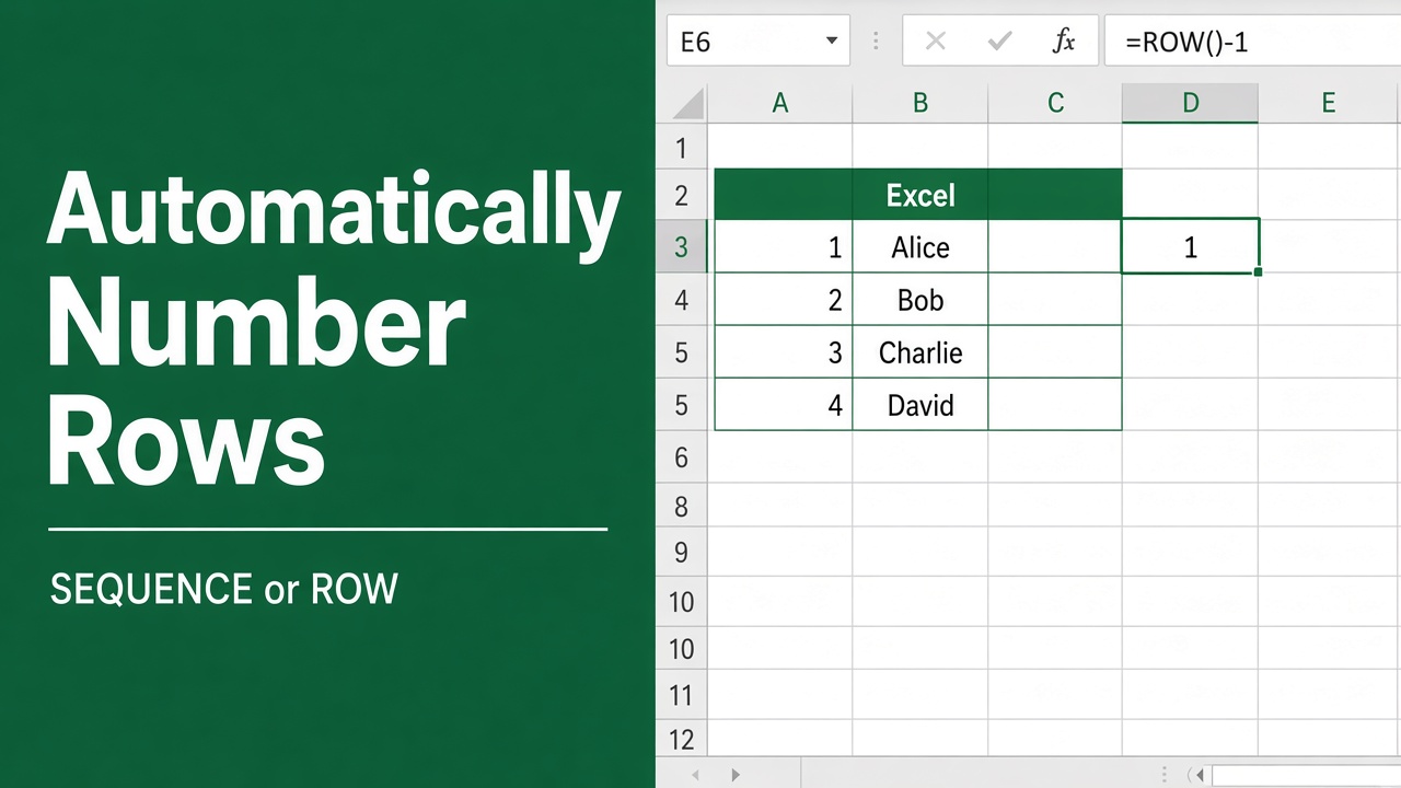
Numbering rows in Excel is something every user eventually needs. Whether you’re organizing a data table, creating a task list, or building a report, having rows automatically numbered saves time and ensures consistency. Instead of typing numbers manually, Excel provides several smart ways to automatically number rows that update dynamically as you add or delete data.
With data starting in row 2, enter =ROW()-1 in A2 and copy it down. The numbers stay in order when you insert or delete rows. In Microsoft 365 or Excel 2021 and later, one formula numbers every filled row in column B and grows as you add data:
=SEQUENCE(COUNTA(B2:B1000))To number only the rows left visible by a filter, use =AGGREGATE(3, 5, B$2:B2) in A2 and copy it down.
In this guide, we will explain multiple methods to number rows automatically in Excel, including formulas, Fill Handle, Excel Tables, and Power Query.
Why Automatically Number Rows in Excel?
Automatically numbering rows helps maintain data order and accuracy. Here’s why it’s useful:
- Ensures consistent row numbering even when sorting or filtering.
- Saves time in large datasets.
- Helps with data analysis and referencing.
- Prevents errors caused by manual entry.
Method 1: Use Fill Handle to Number Rows Automatically
The Fill Handle is one of the simplest ways to create an automatic numbering sequence in Excel.
Steps to Use the Fill Handle
- In cell A2, type
1. - In cell A3, type
2. - Select both cells (A2:A3).
- Hover your mouse over the bottom-right corner until you see the small plus sign (+).
- Drag the Fill Handle down to automatically fill the sequence.
Excel detects the pattern and continues numbering sequentially (3, 4, 5, etc.).
Pros and Cons
| Pros | Cons |
|---|---|
| Quick and easy to use | Does not auto-update when rows are inserted or deleted |
| Works for small datasets | Requires manual adjustment if data changes |
Method 2: Use the ROW Function
The ROW function in Excel is a dynamic way to automatically number rows that updates even when you insert or delete rows.
Basic Formula
If your data starts in row 2, enter this formula in A2:
=ROW()-1This subtracts 1 because the data starts from the second row.
Explanation
ROW()returns the current row number.- Subtracting
1adjusts the numbering to start from 1 instead of 2.
Example
| Row | Formula | Output |
|---|---|---|
| 2 | =ROW()-1 | 1 |
| 3 | =ROW()-1 | 2 |
| 4 | =ROW()-1 | 3 |
Now, if you insert a new row between rows 3 and 4, Excel will automatically update the numbering.
When to Use
Use this method when your data changes frequently or when working with dynamic ranges.
Method 3: Use the SEQUENCE Function (Dynamic Arrays)
If you’re using Excel 365 or Excel 2021, you can take advantage of the SEQUENCE function to generate automatic numbering.
Formula Example
In cell A2, enter:
=SEQUENCE(COUNTA(B2:B100))Here, B2:B100 represents your data range.
How It Works
COUNTA(B2:B100)counts how many rows have data.SEQUENCE()generates that many numbers in order.
The result is a dynamic list of row numbers that automatically expands or contracts as you add or remove data.
Example Output
| A | B |
|---|---|
| 1 | Apple |
| 2 | Banana |
| 3 | Cherry |
| 4 | Date |
Whenever you add another fruit name, Excel automatically generates the next number.
Method 4: Use Excel Table with Structured References
Excel Tables are great for dynamic data management, and they automatically expand as you add new rows.
Steps to Create an Excel Table
- Select your dataset.
- Press Ctrl + T to convert it into a Table.
- In the first column, enter this formula:
=ROW()-ROW(Table1[#Headers])Replace Table1 with your table’s actual name.
How It Works
- The
ROW()function calculates the current row number. - Subtracting
ROW(Table1[#Headers])ensures numbering starts from 1 under the header row.
Benefits
- Automatically updates numbering when you add or delete rows.
- Works well for structured data entry forms or reports.
Method 5: Use Power Query for Advanced Row Numbering
For large datasets or when cleaning imported data, Power Query offers a robust solution.
Steps to Add Index Column in Power Query
- Select your data range and go to the Data tab.
- Choose Get & Transform Data → From Table/Range.
- In the Power Query Editor, go to Add Column → Index Column → From 1.
- Click Close & Load to bring the data back to Excel.
Now your dataset includes a dynamic index column that numbers each row automatically.
Pros
- Ideal for data transformation tasks.
- Handles large datasets efficiently.
- Automatically updates when you refresh the query.
Method 6: Using a Helper Column with IF and COUNTA
You can combine IF, COUNTA, and ROW functions to create numbering that adjusts dynamically when rows are blank or filtered.
Formula Example
In A2, enter:
=IF(B2<>"",COUNTA($B$2:B2),"")Explanation
B2<>""checks if the row has data.COUNTA($B$2:B2)counts how many cells are filled up to that point.- If a cell is empty, Excel leaves the number cell blank.
Output Example
| Row | Data | Formula Output |
|---|---|---|
| 2 | Apple | 1 |
| 3 | Banana | 2 |
| 4 | (empty) | |
| 5 | Cherry | 3 |
This method is useful when your dataset has gaps or empty rows.
Method 7: Automatically Number Rows After Filtering
When you filter data, ROW-based numbers keep their gaps (1, 2, 5, 9...). To renumber only the visible rows 1, 2, 3..., use AGGREGATE, which can ignore hidden rows.
Formula Example
With your data in column B starting at B2, enter this in A2 and copy it down:
=AGGREGATE(3, 5, B$2:B2)Explanation
3tells AGGREGATE to use COUNTA, so it counts non-empty cells.5tells it to ignore hidden rows, including rows hidden by a filter.B$2:B2grows by one row each time the formula is copied down, so each row counts the visible entries above it and itself.
This approach ensures your numbering reflects only visible rows after filters are applied. Point the range at a column that is never blank, and not at the numbering column itself, which would create a circular reference. AGGREGATE works in Excel 2010 and later.
Comparison of Methods to Auto Number Rows in Excel
| Method | Dynamic Update | Works with Filters | Best For |
|---|---|---|---|
| Fill Handle | No | No | Small datasets |
| ROW Function | Yes | No | Basic dynamic lists |
| SEQUENCE Function | Yes | No | Excel 365 users |
| Excel Table | Yes | No | Structured data |
| Power Query | Yes | Yes | Large datasets |
| IF + COUNTA | Yes | No | Skipping blank rows |
| AGGREGATE | Yes | Yes | Filtered data |
Bonus Tip: Convert Numbers to Static Values
If you want to lock the numbering (so it doesn’t change with sorting or editing), you can convert formulas into static numbers.
Steps
- Select the numbered cells.
- Press Ctrl + C to copy.
- Right-click → Paste Special → Values.
Now the numbers are static, preventing accidental changes.
Common Issues and Fixes
| Problem | Cause | Solution |
|---|---|---|
| Numbers disappear when sorting | Formula references moved | Use structured references or Excel Tables |
| Sequence restarts after blank row | Formula depends on adjacent data | Use IF + COUNTA formula |
| Dynamic numbering doesn’t update | Formula not set to dynamic | Use ROW or SEQUENCE |
| Incorrect numbering in filtered list | Hidden rows counted | Use AGGREGATE (Method 7) |
Best Practices for Numbering Rows in Excel
- Use structured references when working with Excel Tables to ensure consistency.
- Avoid hardcoding numbers; use formulas that adjust dynamically.
- Protect formula columns to prevent accidental edits.
- Combine numbering with filters and sorting for cleaner reporting.
- Test formulas after inserting or deleting rows to confirm they auto-adjust.
Final Thoughts
Automatically numbering rows in Excel is an essential data management skill. From simple Fill Handle sequences to advanced Power Query indexing, Excel offers several ways to number rows efficiently.
For small datasets, the ROW or SEQUENCE function works best. For filtered lists, the AGGREGATE formula renumbers only the visible rows.
FAQs
How can I automatically number rows in Excel?
Use dynamic formulas like =ROW()-1, the SEQUENCE function (Excel 365/2021), convert the range to an Excel Table, or add an Index column in Power Query for automatic numbering.
How do I keep row numbers correct after sorting data?
Use structured references inside an Excel Table or add an Index column in Power Query; both keep numbers tied to rows and update when you sort.
How do I number only the visible rows after applying a filter?
Enter =AGGREGATE(3, 5, B$2:B2) in the first row and copy it down. It counts only visible, non-empty cells in column B, so the numbers restart at 1, 2, 3 after filtering.
How can I start numbering from a number other than 1?
Adjust your formula. For example, =ROW()-1+100 starts numbering from 101, or use SEQUENCE with a start argument like =SEQUENCE(n,1,101,1).
How do I convert dynamic numbers into static values?
Select the numbered cells, copy them, then use Paste Special → Values to replace formulas with static numbers that won’t change.
How do I avoid numbering blank rows or skip empty cells?
Use a conditional formula such as =IF(B2<>"",COUNTA($B$2:B2),"") so numbers appear only for rows that contain data in the target column.