
Excel library
Conditional Formatting with Icon Sets in Excel (Easy Guide)
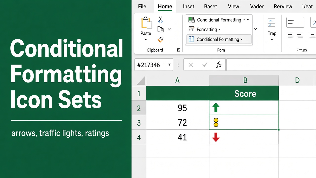
Conditional Formatting with Icon Sets in Excel offers a simple way to turn raw data into visual indicators. Whether you’re showing performance levels, progress tracking, or status checks, icon sets help you communicate information clearly without using extra words or charts.
- Select the numbers, go to Home > Conditional Formatting > Icon Sets, and pick a set.
- To control the cut-offs, open Conditional Formatting > Manage Rules > Edit Rule, change Type to Number, and enter your thresholds (e.g. green when >= 80, yellow when >= 70).
Icon sets only work on numbers. For text such as “Done” or “Pending”, add a helper column that turns it into 1, 2 or 3 and apply the icon set there with Show Icon Only.
In this guide, we will explain how to use, customize, and apply icon sets in Excel, including how to base them on values from other cells. Let’s walk through each step.
What Are Icon Sets in Excel?
Icon Sets are one of the conditional formatting tools that allow you to place symbols in cells based on their values. These symbols can include:
- Arrows
- Flags
- Shapes
- Check marks
- Ratings (stars, bars, etc.)
They automatically group your data into categories (typically 3 to 5 levels), helping you spot trends or conditions quickly. These icons adjust based on value comparisons within a range.
How to Apply Icon Sets in Excel
Let’s look at how to use Excel’s built-in icon set formatting in a worksheet.
Step 1: Select the Range
Click and drag to highlight the cells you want to format with icon sets. This could be a column of scores, percentages, or totals.
Step 2: Open the Conditional Formatting Menu
- Go to the Home tab in the Excel ribbon.
- Click Conditional Formatting in the ‘Styles’ group.
Step 3: Choose an Icon Set
- Hover over Icon Sets.
- Choose a category like:
- Directional (arrows)
- Shapes (traffic lights, circles)
- Indicators (flags, signs)
- Ratings (stars, bars)
Once selected, Excel will apply the icon set based on the default rules.
Customizing Icon Set Rules
Excel uses default thresholds, but you can change them to better fit your data or use case.
How Excel Sets Defaults
By default, Excel splits the range between the lowest and highest value into equal bands, using Percent thresholds:
- 3 icons: top icon at 67% of the range or more, middle at 33% or more
- 4 icons: 75%, 50% and 25%
- 5 icons: 80%, 60%, 40% and 20%
These are percentages of the value range, not equal numbers of cells. One very high or low value can push most cells into the same icon, which is why setting your own Number thresholds is usually better.
But this default behavior doesn’t always fit what you need.
Step-by-Step Customization
- After selecting your icon set, open:
Conditional Formatting > Manage Rules > Edit Rule - In the dialog box, adjust:
- Type (Number, Percent, Formula, or Percentile)
- Values/Thresholds
- Icons (you can change or remove them)
Example: Custom Thresholds
| Value Range | Icon Type |
|---|---|
| ≥ 80 | Green Check |
| 70–79 | Yellow Dash |
| < 70 | Red Cross |
You can apply the rules using “More Rules” and choosing “Number” as the type.
Show Icon Only
To display only the icon (and hide the cell value):
- Check “Show Icon Only” in the rule settings.
Using Icon Sets Based on Another Cell’s Value
Excel doesn’t directly allow icon sets to reference another cell. But you can emulate this behavior with a helper column.
Example: Flag Icon Based on Payment Status
Suppose column D has payment dates.
In column A, enter a formula like:
=IF($D2<>"", 3, 1)This returns:
- 3 if paid (cell has a date)
- 1 if not paid (cell is empty)
Now, apply an icon set to column A.
| Value | Icon |
|---|---|
| 3 | Green Flag |
| 1 | Red Flag |
Check “Show Icon Only” so only the flag shows in column A.
This is useful for dashboards or overviews that reflect status indicators.
Creating Custom Icon Sets Using Formulas and Symbols
If the built-in icons don’t fit, a formula can return a symbol directly. UNICHAR (Excel 2013 and later) works with any normal font, so there is no Wingdings guesswork:
=IF(C5>80, UNICHAR(10004), IF(C5<60, UNICHAR(10008), "!"))Symbol Codes
| Formula | Symbol | Description |
|---|---|---|
UNICHAR(10004) | ✔ | Check mark |
UNICHAR(10008) | ✘ | Cross mark |
UNICHAR(9650) / UNICHAR(9660) | ▲ / ▼ | Up / down arrow |
UNICHAR(9679) | ● | Filled circle |
Color the symbols with ordinary conditional formatting rules, for example green font when C5 > 80. If you prefer the Wingdings font, the check mark is CHAR(252) and the cross CHAR(251); letters like J, K and L show faces in Wingdings, not checks.
Common Use Cases for Icon Sets
Icon sets aren’t just for numbers. They are highly useful in tracking different types of data visually.
1. Performance Indicators
For example, categorize employee performance as:
| Score Range | Icon |
|---|---|
| ≥ 90 | Green Arrow |
| 70–89 | Yellow Arrow |
| < 70 | Red Arrow |
2. Project Progress Tracking
| Completion % | Icon |
|---|---|
| ≥ 90% | Full Circle |
| 50–89% | Half Circle |
| < 50% | Empty Circle |
This helps highlight progress visually across tasks or team members.
3. Risk Assessment
Use arrows or signs to show the direction of risk:
- Up arrow for improving
- Side arrow for stable
- Down arrow for declining
4. Status Checks
Show yes/no or complete/pending conditions using:
- Green check for done
- Red cross for not done
How to Combine Icon Sets with Other Conditional Formatting Rules
You can layer icon sets with:
- Color scales for gradients
- Data bars for progress bars
- Text rules (e.g., format if text contains “urgent”)
This makes your Excel file more dynamic and readable, especially in dashboards and reports.
Summary Table: Quick Steps and Features
Here’s a snapshot of the key steps and how they work:
| Task | Steps |
|---|---|
| Apply icon set | Home > Conditional Formatting > Icon Sets |
| Customize thresholds/icons | Icon Sets > More Rules |
| Show icon only | In More Rules dialog, check “Show Icon Only” |
| Base icons on another cell | Use a helper column with a formula, apply icon set to helper column |
| Custom icons (symbols) | Use CHAR() formula + Wingdings font or insert symbols manually |
Final Thoughts
Icon sets in Excel are a fast and effective way to communicate the status, trends, or performance of your data. By using custom thresholds, helper columns, and symbol-based formulas, you can go beyond the basics and build visuals that bring clarity to your spreadsheets.
For best results, combine icon sets with clear labels, consistent formatting, and a solid understanding of your data goals.
FAQs
How can I apply icon sets to a range of cells?
Select your data range, go to the Home tab, click on Conditional Formatting, choose Icon Sets, and select a style. Excel will automatically apply the icon set based on default rules.
Can I customize icon set thresholds in Excel?
Yes, you can customize the thresholds by going to Conditional Formatting > Manage Rules > Edit Rule. From there, you can set custom values, percentages, or formulas for each icon level.
How do I apply conditional formatting with icon sets using a formula?
Excel does not allow direct use of formulas in icon sets, but you can simulate it by using a helper column that returns values based on your formula. Then apply icon formatting to that helper column.
Can I use icon sets based on text values in Excel?
Yes, you can use a helper column that converts text values to numbers using formulas like =IF(A1=”Completed”,3,IF(A1=”In Progress”,2,1)), and then apply icon sets to the numeric values.
How do I set icon sets based on percentage values?
When setting up your rule, change the type from “Percent” to “Number” if your values are in actual percent format (e.g., 0.8 for 80%). Set thresholds accordingly, such as 0.8, 0.7, etc.
Can Excel icon sets support more than 3 categories?
Yes, Excel provides icon sets with 3, 4, and 5 icons. When you select a set with more than 3 icons, Excel automatically divides the data into equal segments unless you customize the thresholds manually.